Support Vector Machines (II)
CISC 484/684 – Introduction to Machine Learning
Sihan Wei
July 8, 2025
Dual Formulation
Recall: Hard-margin SVM
Primal Problem
\[ \begin{gathered} \min _{w, b} \frac{1}{2}\|w\|^2 \\ \text { s.t. } \quad y_i\left(w^T x_i+b\right) \geq 1, i=1, \ldots, n \end{gathered} \]
Dual Formulation for SVM
We first write out the Lagrangian:
\[ L(\mathbf{w}, b, \alpha)=\frac{1}{2}\|\mathbf{w}\|^2-\sum_{i=1}^n \alpha_i\left\{y_i\left(\mathbf{w} \cdot \mathbf{x}_i+b\right)-1\right\} \]
Then take derivative with respect to \(b\), as it is easy!
\[ \frac{\partial L}{\partial b}=-\sum_{i=1}^n \alpha_i y_i \]
Setting it to 0 , solves for the optimal \(b\), which is a constraint on the multipliers
\[ 0=\sum_{i=1}^n \alpha_i y_i \]
Then take derivative with respect to w :
\[ \frac{\partial L}{\partial w_j}=w_j-\sum_{i=1}^n \alpha_i y_i x_{i, j} \]
\[ \frac{\partial L}{\partial \mathbf{w}}=\mathbf{w}-\sum_{i=1}^n \alpha_i y_i \mathbf{x}_i \]
Setting it to 0 , solves for the optimal w :
\[ \mathbf{w}=\sum_{i=1}^n \alpha_i y_i \mathbf{x}_i \]
Then we now can use these as constraints and obtain a new objective:
\[ \tilde{L}(\alpha)=\sum_{i=1}^n \alpha_i-\frac{1}{2} \sum_{i=1}^n \sum_{j=1}^n \alpha_i \alpha_j y_i y_j \mathbf{x}_i^\top \mathbf{x}_j \]
- Do not forget we have constraints as well
- We are minimizing the dual problem
\[ \tilde{L}(\alpha)=\sum_{i=1}^n \alpha_i-\frac{1}{2} \sum_{i=1}^n \sum_{j=1}^n \alpha_i \alpha_j y_i y_j \mathbf{x}_i^\top \mathbf{x}_j \]
- Subject to:
\[ \begin{gathered} \alpha_i \geq 0 \quad \forall i \\ \sum_{i=1}^n \alpha_i y_i=0 \end{gathered} \]
KKT Conditions
- Under proper conditions there exists a solution
\[ \mathbf{w}^*, \alpha^*, \beta^* \]
- such that the primal and dual have the same solution
\[ d^*=\mathcal{L}\left(\mathbf{w}^*, \alpha^*, \beta^*\right)=p^* \]
- These parameters satisfy the KKT conditions
Sufficient conditions: \(f\) and \(g\) are convex, \(h\) are affine. Then there exists a solution; moreover p* \(=\) \(\mathrm{d}^*\) and the following Karush-Kuhn-Tucker (KKT) conditions hold:
\[ \begin{gathered} \frac{\partial}{\partial w_i} \mathcal{L}\left(\mathbf{w}^*, \alpha^*, \beta^*\right)=0, i=1, \ldots, m \\ \frac{\partial}{\partial \beta_i} \mathcal{L}\left(\mathbf{w}^*, \alpha^*, \beta^*\right)=0, i=1, \ldots, l \\ \alpha_i^* g_i\left(\mathbf{w}^*\right)=0, i=1, \ldots, n \\ g_i\left(\mathbf{w}^*\right) \leq 0, i=1, \ldots, n \\ \alpha_i^* \geq 0, i=1, \ldots, n \end{gathered} \]
Dual vs Primal Formulation
- In the primal we have \(d\) variables to solve
- Solve for the vector \(w\) (length of features)
- In the dual we have \(n\) variables to solve
- Solve for the vector \(\alpha\) (length of examples)
- When to use the primal?
- Lots of examples without many features
- When to use the dual?
- Lots of features without many examples
Practice Question
If you’re training an SVM on 100 images (each 10000 pixels), which form would be more efficient?
Answer: dual, because \(d = 10000\), \(n = 100\) → better to solve in example space.
Soft-margin SVM
Non-separable Data
- But not all data is linearly separable
- What will SVMs do?
- The regularization forces the weights to be small
- But it must still find a max margin solution
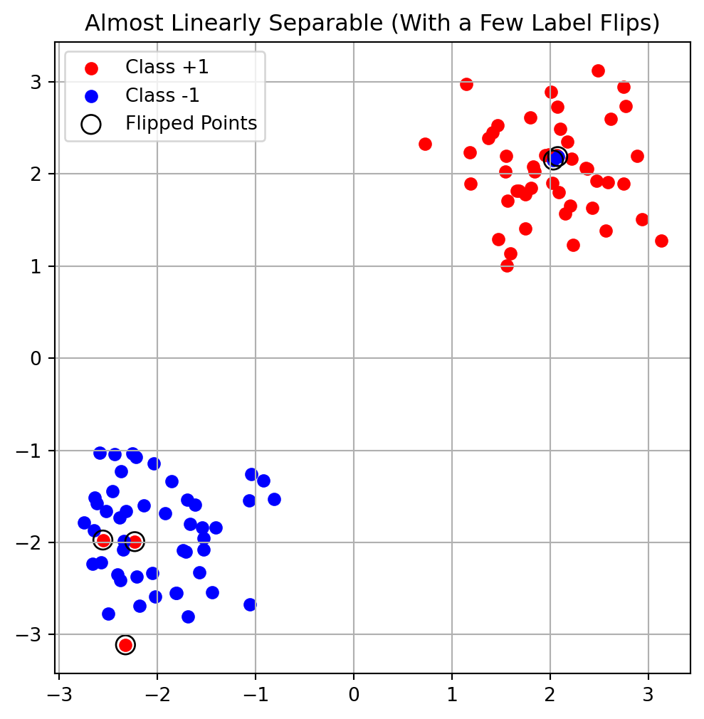
- Idea: for every data point, we introduce a slack variable. The value is the distance of the data from the corresponding class’s margin if it is on the wrong side of the margin, otherwise zero.
Example: Non-linearly Separable data in 2D
Slack Variables
For each of the \(n\) training examples, we will introduce an non-negative variable \(\xi_i\), and the optimization problem becomes:
\[ \begin{aligned} & \quad \min _{\mathbf{w}} \frac{1}{2}\|\mathbf{w}\|_2^2+C \sum_{i=1}^n \xi_i \quad \text { such that } \\ & \forall i, \quad y_i\left(\mathbf{w}^{\top} x_i\right) \geq 1-\xi_i \\ & \forall i, \quad \xi_i \geq 0 \end{aligned} \]
This is also called the soft-margin SVM.
Note that \(\xi_i /\|\mathbf{w}\|_2\) is the distance the example \(i\) need to move to satisfy the constraint \(y_i\left(\mathbf{w}^{\top} x_i\right) \geq 1\).
- \(C\) is a hyperparameter controlling how many points we allow to violate the margin constraint.
- We can always satisfy the margin using \(\xi\)
- We want these \(\xi\) to be small
- Trade off parameter \(C\)
Dual Derivation for Soft-Margin SVM
- We introduce slack variables \(\xi_i\) for soft-margin violations.
- The Lagrangian becomes:
\[ \begin{aligned} \mathcal{L}(w, b, \boldsymbol{\alpha}, \boldsymbol{\xi}, \boldsymbol{\mu}) &= \frac{1}{2} \|w\|^2 + C \sum_{i=1}^n \xi_i \\ &\quad- \sum_{i=1}^n \alpha_i \left( y_i(w^\top x_i + b) - 1 + \xi_i \right) \\ &\quad- \sum_{i=1}^n \mu_i \xi_i \end{aligned} \]
Solving the Lagrangian
- Taking derivatives and setting to 0 gives the same dual objective as in hard-margin:
\[ \sum_{i=1}^n \alpha_i - \frac{1}{2} \sum_{i=1}^n \sum_{j=1}^n \alpha_i \alpha_j y_i y_j \langle x_i, x_j \rangle \]
- But with different constraints:
\[ \frac{\partial \mathcal{L}}{\partial \xi_i} = 0 \quad \Rightarrow \quad \alpha_i + \mu_i = C \]
- Thus, we obtain:
\[ 0 \le \alpha_i \le C \]
Soft Margin
- Points that are far away from the margin on the wrong side would get more penalty.
- All misclassified examples will be support vectors
- All points “crossed” the margin line will be support vectors
\[ \alpha_i^* g_i\left(\mathbf{w}^*\right)=0, i=1, \ldots, n \]
Bias VS Variance
- Smaller C means more slack (larger \(\xi\))
- More training examples are wrong
- More bias (less variance) in the output
- Larger C means less slack (smaller \(\xi\))
- Better fit to the data
- Less bias (more variance) in the output
- For non-separable data we can’t learn a perfect separator so we don’t want to try too hard
- Finding the right balance is a tradeoff
Support Vectors
The Role of Lagrange Multipliers
In the SVM framework, each training data point is associated with a Lagrange multiplier, denoted as \(\alpha_i\). The decision boundary is computed as:
\[ \mathbf{w}^* = \sum_{i=1}^n \alpha_i y_i \mathbf{x}_i \]
Only those data points for which \(\alpha_i > 0\) contribute to this sum. In other words, if a data point’s corresponding multiplier is zero, it has no impact on the decision boundary. These influential points are what we call support vectors.
Support Vectors in Hard-Margin SVM
For datasets that are perfectly separable, we use a hard-margin SVM. Here, the complementary slackness condition tells us:
\[ \alpha_i(1 - y_i\mathbf{w}^\top\mathbf{x}_i) = 0 \]
This equation means that for points not on the margin (where \(y_i\mathbf{w}^\top\mathbf{x}_i > 1\)), the multiplier \(\alpha_i\) must be 0. Hence, only those points that lie exactly on the margin (where \(y_i\mathbf{w}^\top\mathbf{x}_i = 1\)) have non-zero multipliers and are thus support vectors.
Support Vectors in Soft-Margin SVM
When data is not perfectly separable, SVMs use a soft-margin approach with slack variables \(\xi_i\). The complementary slackness and KKT conditions become:
\[ \alpha_i(1 - y_i\mathbf{w}^\top\mathbf{x}_i - \xi_i) = 0 \\ (C - \alpha_i)\xi_i = 0 \]
We then encounter two cases:
\(\alpha_i > 0\), \(\xi_i = 0\): The point lies exactly on the margin border. It is a support vector.
\(\alpha_i > 0\), \(\xi_i > 0\): The point is either inside the margin or misclassified. Here, \(\alpha_i = C\). These points also influence the decision boundary and are support vectors.
In contrast, points with \(\alpha_i = 0\) lie far from the margin and do not affect the model.
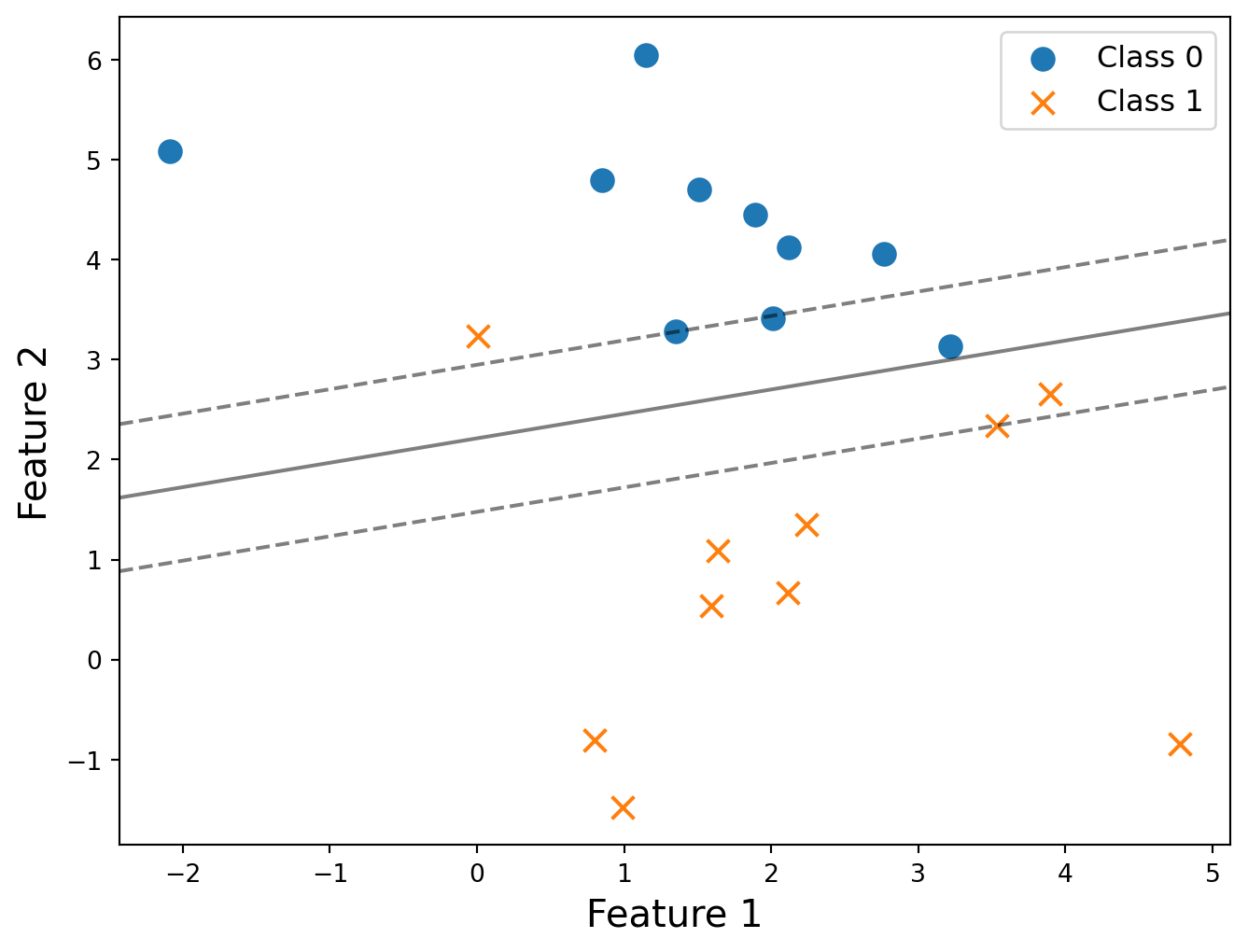
Practice Questions (I)
- How many support vectors in this plot? Circle all of them.
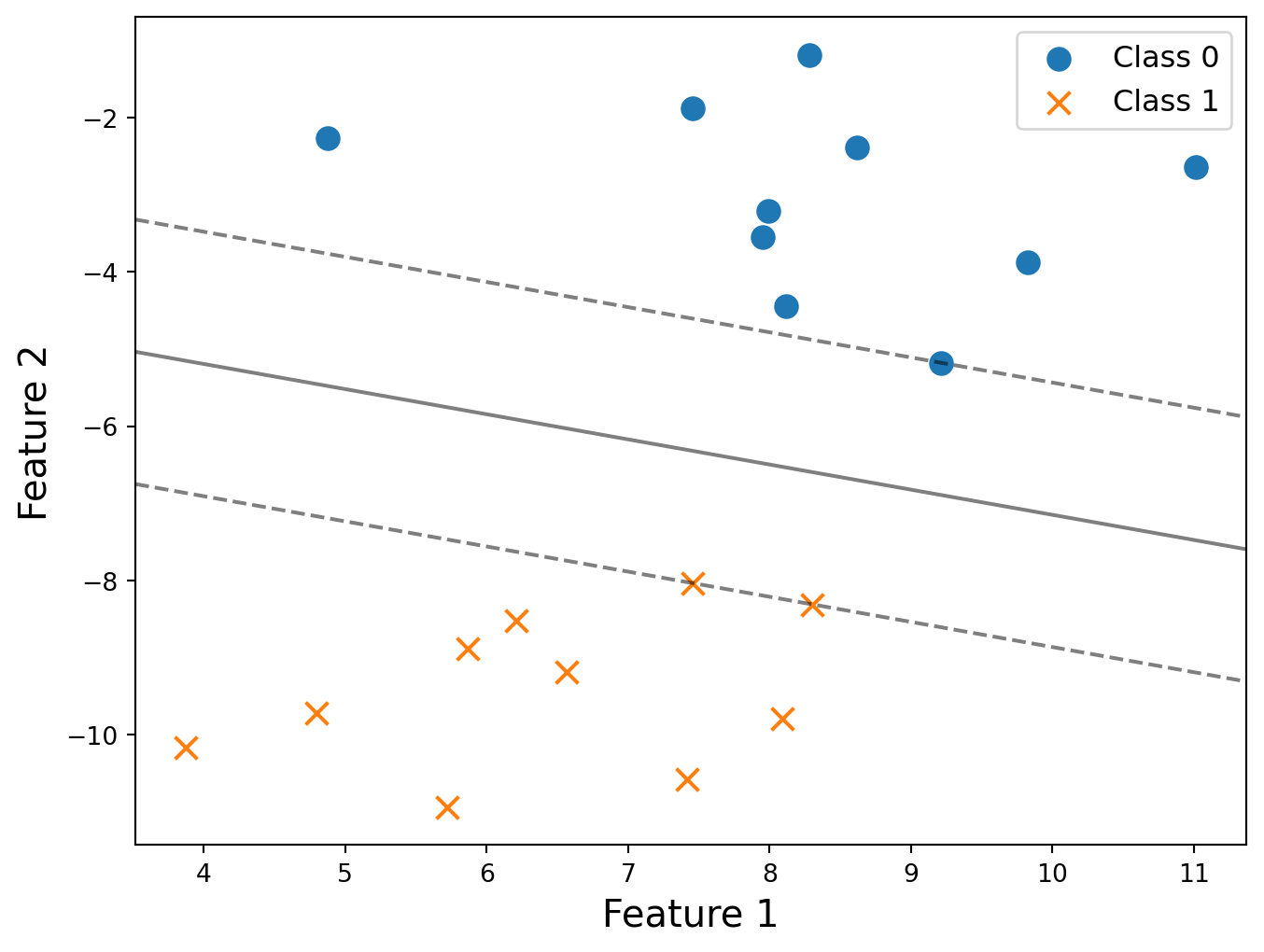
The number of suppost vectors is 3.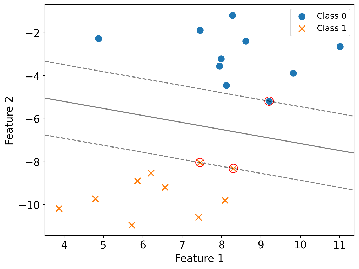
In hard-margin SVM, only the data points that lie exactly on the margin boundaries are support vectors.
Practice Question (II)
- How many support vectors in this plot? Circle all of them.
The number of support vectors is 6.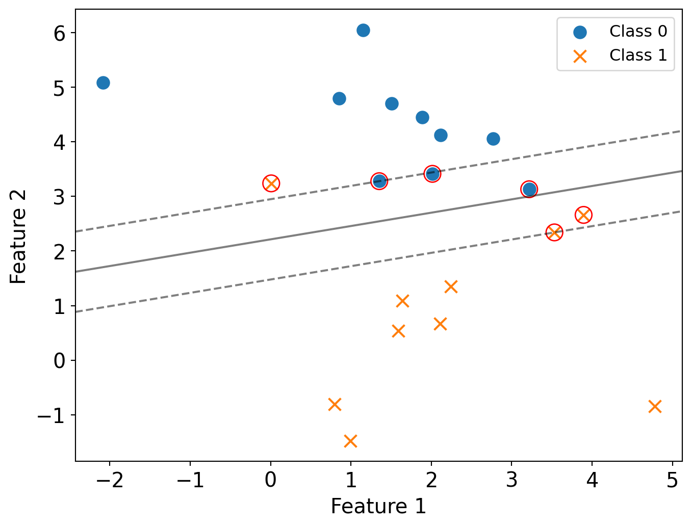
In the soft-margin setting, support vectors are:
- Points lying exactly on the margin boundaries
- Points that are within the margin
- Points that are misclassified (on the wrong side of the decision boundary)
Kernels
How to deal with non linearly separable data
- Option 1: Add features by hand that make the data separable
- Requires feature engineering
- Option 2: Soft-margin and trade off bias and variance
- Option 3: transform to a different feature space by using feature mapping functions
Example: XOR Dataset
- It is linearly non-separable in the 2D space.
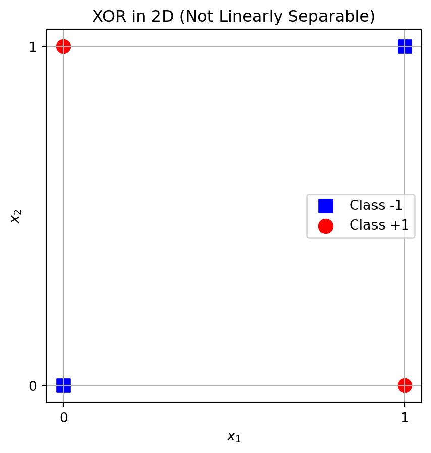
What’s the fix?
To separate XOR using a linear hyperplane, we need to lift it to a higher-dimensional feature space like:
\[ \phi(x)=\left(x_1, x_2, x_1 \cdot x_2\right) \]
Then in 3D space with this embedding, we can separate the classes using a linear function
For example, let’s try:
\[ f(x)=-1+2 x_1+2 x_2-4 x_1 x_2 \]
Plug it in for all 4 points:
| Point | \(f(x)\) | Label |
|---|---|---|
| (0,0) | -1 | -1 ✅ |
| (0,1) | +1 | +1 ✅ |
| (1,0) | +1 | +1 ✅ |
| (1,1) | -1 | -1 ✅ |
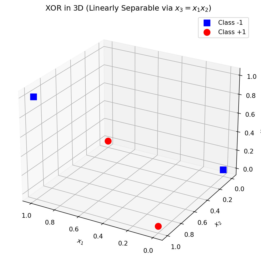
XOR in 3D with Lifted Feature \(x_3 = x_1 x_2\)
- The dataset is linearly separable in 3D.
Key Observations
\[ \boldsymbol{x}^T \cdot \boldsymbol{w}=\boldsymbol{x}^T \cdot \sum_{i=1}^n\left[\alpha_i \boldsymbol{y}_i \boldsymbol{x}_i\right]=\sum_{i=1}^n \alpha_i \boldsymbol{y}_i\left(\boldsymbol{x}^T \cdot \boldsymbol{x}_i\right) \]
- Our prediction is only dependent on the dot product of data or the product of features!
\[ x^T \cdot w=\sum_1^n \alpha_i y_i\left(\phi(x) \cdot \phi\left(x_i\right)\right) \]
Kernels
- Let’s replace \(\phi\left(\boldsymbol{x}_i\right) \phi\left(\boldsymbol{x}_j^T\right)\) with a kernel function K
\[ \sum_{i=1}^n \alpha_i-\frac{1}{2} \sum_{i=1}^n \sum_{j=1}^n y_i y_j \alpha_i \alpha_j K\left(x_i, x_j\right) \]
- where
\[ \boldsymbol{x}^T \cdot \boldsymbol{w}=\boldsymbol{x}^T \cdot \sum_{i=1}^n\left[\alpha_i \boldsymbol{y}_i \boldsymbol{x}_i\right]=\sum_{i=1}^n \alpha_i \boldsymbol{y}_i K\left(\boldsymbol{x}, \boldsymbol{x}_i\right) \]
\[ K\left(x, x^{\prime}\right)=\left(\phi(x) \phi\left(x^{\prime}\right)^T\right) \]
Why?
- We have removed all dependencies in the SVM on the size of the feature space
- The feature space \(\phi(x)\) appears only in the kernel
- As long as the Kernel function does the work, we can handle any feature space
Definition
A kernel function \(K: \mathcal{X} \times \mathcal{X} \rightarrow \mathbb{R}\) is a symmetric function such that for any \(x_1, x_2, \ldots, x_n \in \mathcal{X}\), the \(n \times n\) Gram matrix \(G\) with each \((i, j)\)-th entry \(G_{i j}=K\left(x_i, x_j\right)\), is positive semidefinite (p.s.d.).
Recall that a matrix \(G \in \mathbb{R}^{n \times n}\) is positive semi-definite if and only if \(\forall q \in \mathbb{R}^n, q^{\top} G q \geq 0\).
How to show \(K\) is a kernel? A
A simple way to show a function \(K\) is a kernel is to find a feature expansion mapping \(\phi\) such that
\[ \phi(x)^{\top} \phi\left(x^{\prime}\right)=K\left(x, x^{\prime}\right) \]
Practice Question
Let \(\mathbf{x} = \begin{bmatrix} x_1 \\ x_2 \end{bmatrix} \in \mathbb{R}^2\) and define: \[ K(\mathbf{x}, \mathbf{z}) = (\mathbf{x}^\top \mathbf{z})^2 \]
Questions:
- Is \(K(\mathbf{x}, \mathbf{z})\) a valid kernel function?
- If so, find a feature map \(\phi : \mathbb{R}^2 \to \mathbb{R}^d\) such that: \[ K(\mathbf{x}, \mathbf{z}) = \phi(\mathbf{x})^\top \phi(\mathbf{z}) \]
Solution
We expand the expression: \[ (\mathbf{x}^\top \mathbf{z})^2 = (x_1 z_1 + x_2 z_2)^2 = x_1^2 z_1^2 + 2x_1x_2 z_1z_2 + x_2^2 z_2^2 \]
This is the same as: \[ \phi(\mathbf{x})^\top \phi(\mathbf{z}) \quad \text{where} \quad \phi(\mathbf{x}) = \begin{bmatrix} x_1^2 \\ \sqrt{2} x_1 x_2 \\ x_2^2 \end{bmatrix} \]
Final Answer:
\[ \phi(\mathbf{x}) = \begin{bmatrix} x_1^2 \\ \sqrt{2} x_1 x_2 \\ x_2^2 \end{bmatrix} \quad \text{maps } \mathbb{R}^2 \to \mathbb{R}^3 \]
So \(K(\mathbf{x}, \mathbf{z})\) is a valid kernel, corresponding to an inner product in feature space.
Kernel Preserving Operations
Suppose \(K_1, K_2\) are valid kernels, \(c \geq 0, g\) is a polynomial function with positive coefficients (that is \(\sum_{j=1}^m \alpha_j x^j\) for some \(m \in \mathbb{N}, \alpha_1, \ldots, \alpha_m \in\) \(\mathbb{R}^{+}\)), \(f\) is any function and matrix \(A \succeq 0\) is positive semi-definite. Then following functions are also valid kernels:
- \(K\left(x, x^{\prime}\right)=c K_1\left(x, x^{\prime}\right)\)
- \(K\left(x, x^{\prime}\right)=K_1\left(x, x^{\prime}\right)+K_2\left(x, x^{\prime}\right)\)
- \(K\left(x, x^{\prime}\right)=g\left(K\left(x, x^{\prime}\right)\right)\)
- \(K\left(x, x^{\prime}\right)=K_1\left(x, x^{\prime}\right) K_2\left(x, x^{\prime}\right)\)
- \(K\left(x, x^{\prime}\right)=f(x) K_1\left(x, x^{\prime}\right) f\left(x^{\prime}\right)\)
- \(K\left(x, x^{\prime}\right)=\exp \left(K_1\left(x, x^{\prime}\right)\right)\)
- \(K\left(x, x^{\prime}\right)=x^{\top} A x^{\prime}\)
You will need to prove one of these properties in homework.
Examples of kernel functions
- Linear: \(K\left(x, x^{\prime}\right)=x^{\top} x^{\prime}\). (Althoug this does not modify the features, it can be faster to pre-compute the Gram matrix when the dimensionality \(d\) of the data is high.)
- Polynomial:
\[ K\left(x, x^{\prime}\right)=\left(1+x^{\top} x^{\prime}\right)^d \]
- Radial Basis Function (RBF) (aka Gaussian Kernel):
\[ K\left(x, x^{\prime}\right)=\exp \left(-\gamma\left\|x-x^{\prime}\right\|^2\right) \]
Example: RBF
- Radial Basis Function (RBF) Kernel (Gaussian Kernel)
\[ K\left(x, x^{\prime}\right)=\exp \left(-\gamma\left\|x-x^{\prime}\right\|^2\right) \]
- \(\gamma\) is the “spread” of the kernel
- Gaussian function in kernel form
Example: RBF
- Why is this a kernel?
- Inner product of two vectors in infinite dimensional space
\[ K\left(x, x^{\prime}\right)=<\psi(x), \psi\left(x^{\prime}\right)> \]
where
\[ \psi: \mathbb{R}^n \rightarrow \mathbb{R}^{\infty} \]
Example: RBF
- What is the RBF kernel measuring?
- Similarity as a decaying function of the distance between the vectors (squared norm of distance)
- Closer vector have smaller difference, and thus the value will be larger ( \(-\gamma\) )
- \(\gamma\) sets the width of the bell shaped curve
- Larger values, narrower bell
\[ K\left(x, x^{\prime}\right)=\exp \left(-\gamma\left\|x-x^{\prime}\right\|^2\right) \]