What Makes a Good Classifier?
There are many lines that separates the data. Which one is the BEST?
- All of these equally separate the data (perfect accuracy)… but are they equally safe?
A Dangerous Point
![]()
- Let’s first try classifier (a)
A Dangerous Point
![]()
- mission failed for classifier (a) 😩
A Dangerous Point
What about classifier (c)
![]()
- Mission success 🥳
- But what makes the difference?
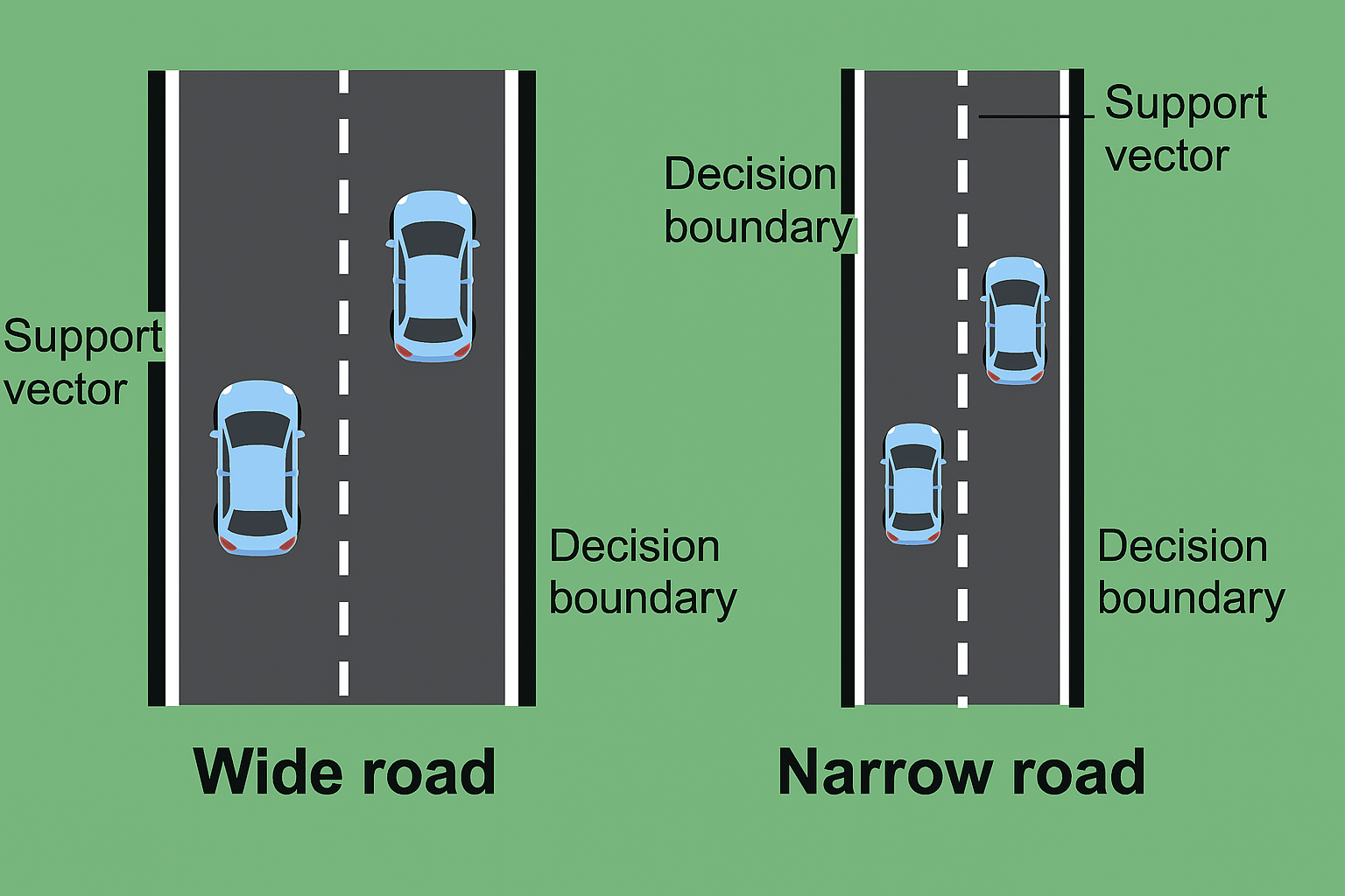
Roads
- Margin is like the buffer zone between classes.
- A wide margin means even if future data wiggles a bit, we’ll probably still classify correctly.
- SVM chooses the boundary that makes the safest, widest road possible.
Geometric margin
- Similar to the idea to the width of a road, we define margin as:
- the distance from the decision boundaries to the closest point across both classes.
- This margin reflects how confidently we can separate the data.
Geometric Margin
- Margin boundaries are parallel to the decision boundary and pass through the support vectors.
- We know we need to maximize the margin now. But how?
Recall: distance from a point to a line
In the case of a line in the plane given by the equation \(a x+b y+c=0\), where \(a, b\) and \(c\) are real constants with \(a\) and \(b\) not both zero, the distance from the line to a point \(\left(x_0, y_0\right)\) is:
\[
\operatorname{distance}\left(a x+b y+c=0,\left(x_0, y_0\right)\right)=\frac{\left|a x_0+b y_0+c\right|}{\sqrt{a^2+b^2}} .
\]
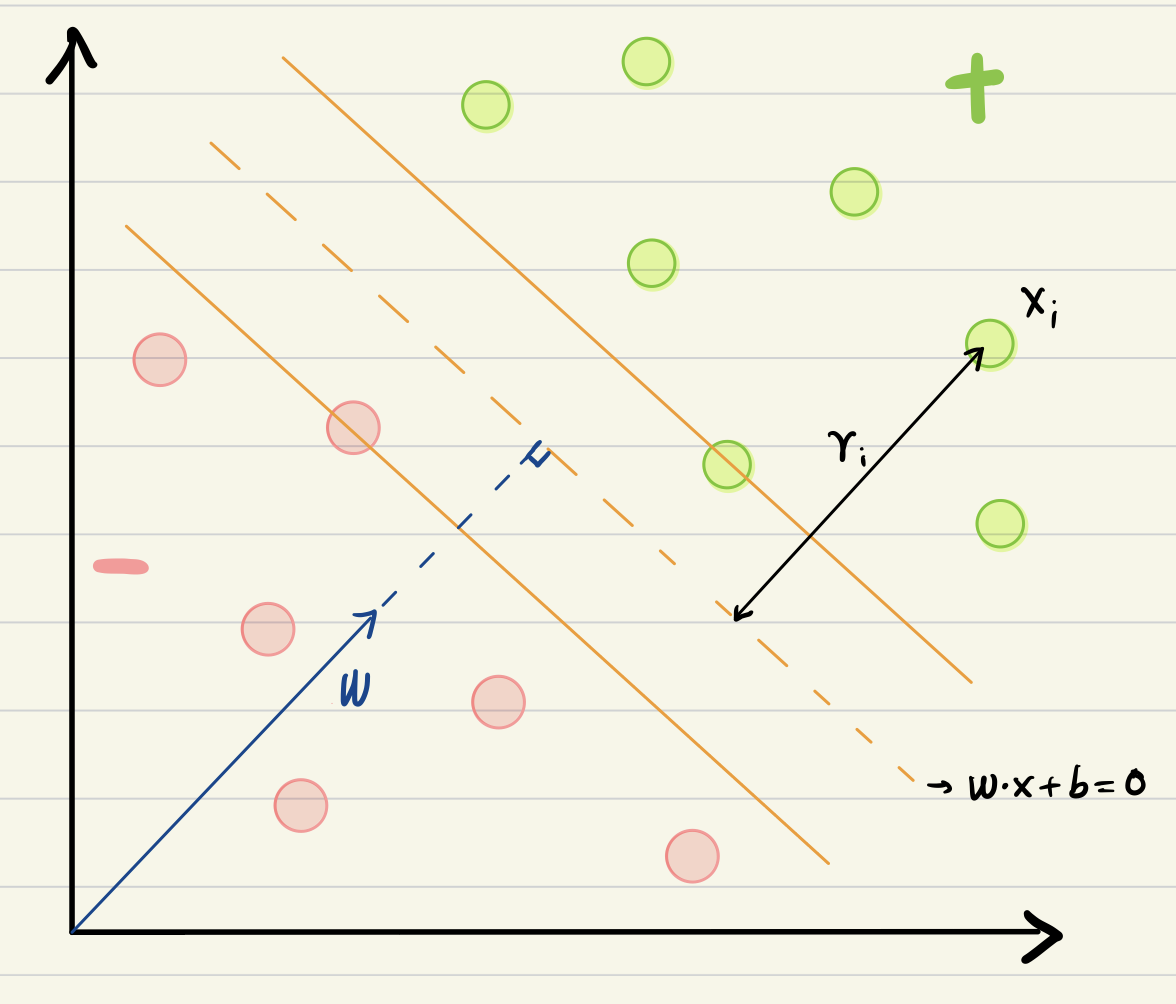
Geometric Representation (I)
For a random point \(x_i\), it’s distance to the decision boundary
\[
r_i=\frac{\left|\vec{w} \cdot \vec{x}_i+b\right|}{\|\vec{w}\|} .
\]
We introduce \(y\) :
\[
\begin{aligned}
& y=+1 \text { for }+ \text { samples } \\
& y=-1 \text { for }- \text { samples } \\
& \gamma_i=y_i\left(\frac{\vec{w} \cdot \vec{x}_i+b}{\|\vec{w}\|}\right)
\end{aligned}
\]
Maximum Geometric Margin
- geometric margin \[
\begin{aligned}
&\gamma_i=y_i\left(\frac{\vec{w} \cdot \vec{x}_i+b}{\|\vec{w}\|}\right)
\end{aligned}
\]
Let’s say each sample has distance at least \(\gamma\), i.e. We constrain \(\gamma_i \geqslant \gamma \forall i\).
And we want to maximize \(\gamma\), i.e. we want points closest to the decision boundary to have large margin.
Objective.
\(\max \gamma\)
s.t. \(\quad \frac{y_i\left(\vec{w} \cdot \vec{x}_i+b\right)}{\|\vec{w}\|} \geqslant \gamma\)
- functional margin \[
\hat{\gamma}_i=\underset{\text { label }}{y_i} \underset{\text { prediction }}{\left(\stackrel{\rightharpoonup}{w} \cdot \stackrel{\rightharpoonup}{x}_i+b\right)}
\]
Objective
\(\max \frac{\hat{\gamma}}{\|\vec{w}\|}\)
s.t. \(y_i\left(\vec{w} \cdot \vec{x}_i+b\right) \geqslant \hat{\gamma}\)
- Notice that the value of \(\hat{\gamma}\) doesn’t matter (why?). We can set it to 1.
\[
\begin{array}{lll}
\max \frac{1}{\|\vec{w}\|} & \Leftrightarrow & \min \frac{1}{2}\|\vec{w}\|^2 \\
\text { s.t. } y_i\left(\vec{w} \cdot \vec{x}_i+b\right) \geqslant 1 & \quad & \text{ s.t. } y_i\left(\vec{w} \cdot \vec{x}_i+b\right) \geqslant 1
\end{array}
\]
- Here we have derived the hard-margin SVM!
Lagrangians for�Constrained Optimization
Problem
\[
\begin{gathered}
\operatorname{minf}_{\mathbf{w}}(\mathbf{w}) \\
\operatorname{s.t.} g_i(\mathbf{w}) \leq 0, i=1, \ldots, n \\
h_j(\mathbf{w})=0, j=1, \ldots, l
\end{gathered}
\]
Define
\[
\mathcal{L}(\mathbf{w}, \alpha, \beta)=f(\mathbf{w})+\sum_{i=1}^n \alpha_i g_i(\mathbf{w})+\sum_{j=1}^l \beta_j h_j(\mathbf{w})
\]
\[
\frac{\partial \mathcal{L}}{\partial w_i}=0
\]
Setting it to 0 , solves for the optimal \(b\), which is a constraint on the multipliers
\[
0=\sum_{i=1}^n \alpha_i y_i
\]
Then take derivative with respect to w :
\[
\frac{\partial L}{\partial w_j}=w_j-\sum_{i=1}^n \alpha_i y_i x_{i, j}
\]
\[
\frac{\partial L}{\partial \mathbf{w}}=\mathbf{w}-\sum_{i=1}^n \alpha_i y_i \mathbf{x}_i
\]
Setting it to 0 , solves for the optimal w :
\[
\mathbf{w}=\sum_{i=1}^n \alpha_i y_i \mathbf{x}_i
\]
Then we now can use these as constraints and obtain a new objective:
\[
\tilde{L}(\alpha)=\sum_{i=1}^n \alpha_i-\frac{1}{2} \sum_{i=1}^n \sum_{j=1}^n \alpha_i \alpha_j y_i y_j \mathbf{x}_i \mathbf{x}_j
\]
- Do not forget we have constraints as well
- We are minimizing
\[
\tilde{L}(\alpha)=\sum_{i=1}^n \alpha_i-\frac{1}{2} \sum_{i=1}^n \sum_{j=1}^n \alpha_i \alpha_j y_i y_j \mathbf{x}_i \mathbf{x}_j
\]
\[
\begin{gathered}
\alpha_i \geq 0 \quad \forall i \\
\sum_{i=1}^n \alpha_i y_i=0
\end{gathered}
\]