Support Vector Machines (I)
CISC 484/684 – Introduction to Machine Learning
Quick Updates
- HW 2 out
- Due July 14th 11:59 PM
- Get started early, as debugging could be time consuming
- Midterm moved to July 17th
- Thursday, in-class
Roadmap
So far
- Supervised Learning
- Regression
- Linear Regression
- Classification
- Logistic Regression
- SVM (today)
- Regression
- Unsupervised Learning
Data Geometry in Classification
How We Represent Data?
- A convenient way to represent data
- We use a data pair \(\left(x_i, y_i\right)\) where \(x_i\) is the data vector and \(y_i\) is its label.
\[ \left\{\left(x_i, y_i\right)\right\}_{i=1}^n \quad \text { where } x_i \in \mathbb{R}^d, y_i \in\{-1,+1\} \]
- How does the data look geometrically?
Geometric Representation
- Each example \(x_i \in \mathbb{R}^d\) represents a point in an \(d\) dimensional space
- Classification: divides space into 2 parts
- Examples labeled according to where they are
- Linear classification
- A linear decision boundary
- A hyper-plane (d-1 dimensions)
Geometric Representation
- Linearly separable data
- can be separated by a line
- Labels or classes:
- Red squares: class 1 or positive
- Blue dots: class -1 or negative

Linear Classifiers
- Logistic regression gives us a probability that we threshold
- What if just learn the line directly?
- Classification boundary represented by \(w\)
- \(w\) is a vector that is orthogonal (normal) to the decision boundary
\[ \hat{y}=\operatorname{sign}(w^\top x) \]
- Note: \(\hat{y}\) is our prediction, while \(y\) is the true label.
- Prediction
- The sign of the prediction, (-1 or 1) indicates which side of the boundary
Multiple Linear classifiers

Margin-based Classifiers
What Makes a Good Classifier?
There are many lines that separates the data. Which one is the BEST?


- All of these equally separate the data (perfect accuracy)… but are they equally safe?
A Dangerous Point

- Let’s first try classifier (a)
A Dangerous Point

- mission failed for classifier (a) 😩
A Dangerous Point
What about classifier (c)

- Mission success 🥳
- But what makes the difference?
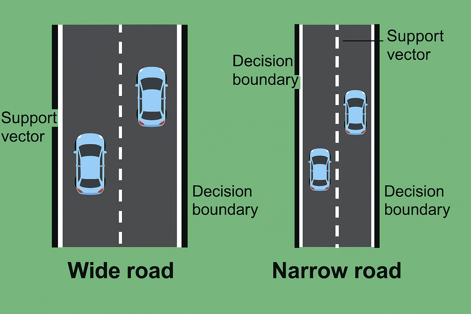
Roads
- Margin is like the buffer zone between classes.
- A wide margin means even if future data wiggles a bit, we’ll probably still classify correctly.
- SVM chooses the boundary that makes the safest, widest road possible.
Geometric margin
- Similar to the idea to the width of a road, we define margin as:
- the distance from the decision boundaries to the closest point across both classes.
- This margin reflects how confidently we can separate the data.

Geometric Margin
- Margin boundaries are parallel to the decision boundary and pass through the support vectors.
- We know we need to maximize the margin now. But how?
Recall: distance from a point to a line
In the case of a line in the plane given by the equation \(a x+b y+c=0\), where \(a, b\) and \(c\) are real constants with \(a\) and \(b\) not both zero, the distance from the line to a point \(\left(x_0, y_0\right)\) is:
\[ \operatorname{distance}\left(a x+b y+c=0,\left(x_0, y_0\right)\right)=\frac{\left|a x_0+b y_0+c\right|}{\sqrt{a^2+b^2}} . \]
Geometric Representation (I)
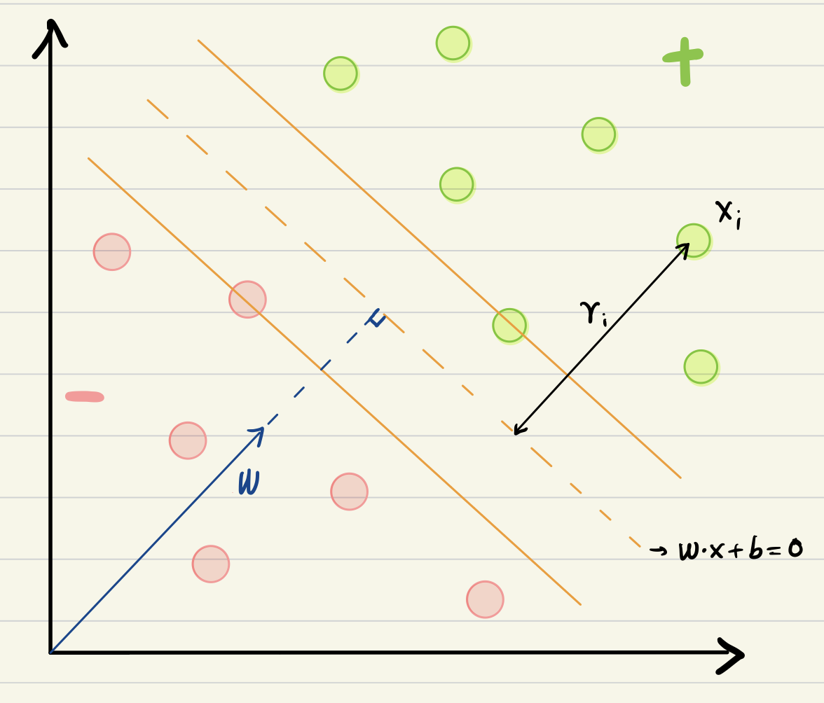
For a random point \(x_i\), it’s distance to the decision boundary
\[ r_i=\frac{\left|\vec{w} \cdot \vec{x}_i+b\right|}{\|\vec{w}\|} . \]
We introduce \(y\) :
\[ \begin{aligned} & y=+1 \text { for }+ \text { samples } \\ & y=-1 \text { for }- \text { samples } \\ & \gamma_i=y_i\left(\frac{\vec{w} \cdot \vec{x}_i+b}{\|\vec{w}\|}\right) \end{aligned} \]
Maximum Geometric Margin
- geometric margin \[ \begin{aligned} &\gamma_i=y_i\left(\frac{\vec{w} \cdot \vec{x}_i+b}{\|\vec{w}\|}\right) \end{aligned} \]
Let’s say each sample has distance at least \(\gamma\), i.e. We constrain \(\gamma_i \geqslant \gamma \forall i\).
And we want to maximize \(\gamma\), i.e. we want points closest to the decision boundary to have large margin.
Objective.
\(\max \gamma\)
s.t. \(\quad \frac{y_i\left(\vec{w} \cdot \vec{x}_i+b\right)}{\|\vec{w}\|} \geqslant \gamma\)
- functional margin \[ \hat{\gamma}_i=\underset{\text { label }}{y_i} \underset{\text { prediction }}{\left(\stackrel{\rightharpoonup}{w} \cdot \stackrel{\rightharpoonup}{x}_i+b\right)} \]
Objective
\(\max \frac{\hat{\gamma}}{\|\vec{w}\|}\)
s.t. \(y_i\left(\vec{w} \cdot \vec{x}_i+b\right) \geqslant \hat{\gamma}\)
- Notice that the value of \(\hat{\gamma}\) doesn’t matter (why?). We can set it to 1.
\[ \begin{array}{lll} \max \frac{1}{\|\vec{w}\|} & \Leftrightarrow & \min \frac{1}{2}\|\vec{w}\|^2 \\ \text { s.t. } y_i\left(\vec{w} \cdot \vec{x}_i+b\right) \geqslant 1 & \quad & \text{ s.t. } y_i\left(\vec{w} \cdot \vec{x}_i+b\right) \geqslant 1 \end{array} \]
- Here we have derived the hard-margin SVM!
Loss minimization interpretation: Hinge loss
SVM vs Logistic Regression
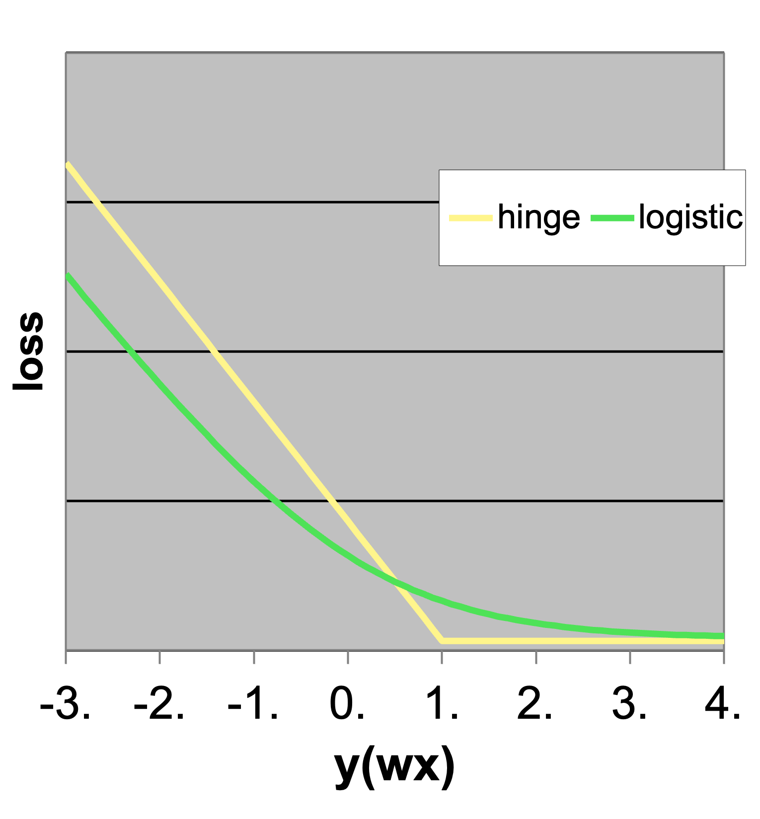
- Logistic loss
\[ \ell_{\text{log}}=\log(1+\exp(-y(w^\top x))) \]
- Hinge Loss
\[ \ell_{\text{hinge}} = \max\{0,1-y(w^\top x)\} \]
- Note the loss function behavior; SVM has a discontinuity at the margin. It “cares a lot” as soon as a point passes the margin.
SVM vs. Logistic Regression
- Both minimize the empirical loss with some regularization
- SVM:
\[ \frac{1}{n} \sum_{i=1}^n\left(1-y_i\left[w \cdot x_i\right]\right)^{+}+\lambda \frac{1}{2}\|w\|^2 \]
- Logistic:
\[ \frac{1}{n} \sum_{i=1}^n \underbrace{-\log g\left(y_i\left[w \cdot x_i\right]\right)}_{-P\left(y_i \mid x_i, w\right)}+\lambda \frac{1}{2}\|w\|^2 \]
- (z)+ indicates only positive values
- \(\mathrm{g}(\mathrm{z})=(1+\exp (-\mathrm{z}))^{-1}\) is the logistic function
Dual Formulation
Lagrangians for Constrained Optimization
Problem
\[ \begin{gathered} \operatorname{minf}_{\mathbf{w}}(\mathbf{w}) \\ \operatorname{s.t.} g_i(\mathbf{w}) \leq 0, i=1, \ldots, n \\ h_j(\mathbf{w})=0, j=1, \ldots, l \end{gathered} \]
Define
\[ \mathcal{L}(\mathbf{w}, \alpha, \beta)=f(\mathbf{w})+\sum_{i=1}^n \alpha_i g_i(\mathbf{w})+\sum_{j=1}^l \beta_j h_j(\mathbf{w}) \]
- Solve
\[ \frac{\partial \mathcal{L}}{\partial w_i}=0 \]
Dual Formulation
- “Primal” and “dual are complimentary solutions of the Lagrangian problem
\[ d^*=\max _{\alpha, \beta: \alpha_i \geq 0} \min _{\mathbf{w}} \mathcal{L}(\mathbf{w}, \alpha, \beta) \leq \min _{\mathbf{w}} \max _{\alpha, \beta: \alpha_i \geq 0} \mathcal{L}(\mathbf{w}, \alpha, \beta)=p^* \]
- This is true by the “Max-min” inequality
- There are some conditions for this to hold, which we will cover in our next lecture!
Dual Formulation for SVM
We first write out the Lagrangian:
\[ L(\mathbf{w}, b, \alpha)=\frac{1}{2}\|\mathbf{w}\|^2-\sum_{i=1}^n \alpha_i\left\{y_i\left(\mathbf{w} \cdot \mathbf{x}_i+b\right)-1\right\} \]
Then take derivative with respect to \(b\), as it is easy!
\[ \frac{\partial L}{\partial b}=-\sum_{i=1}^n \alpha_i y_i \]
Setting it to 0 , solves for the optimal \(b\), which is a constraint on the multipliers
\[ 0=\sum_{i=1}^n \alpha_i y_i \]
Then take derivative with respect to w :
\[ \frac{\partial L}{\partial w_j}=w_j-\sum_{i=1}^n \alpha_i y_i x_{i, j} \]
\[ \frac{\partial L}{\partial \mathbf{w}}=\mathbf{w}-\sum_{i=1}^n \alpha_i y_i \mathbf{x}_i \]
Setting it to 0 , solves for the optimal w :
\[ \mathbf{w}=\sum_{i=1}^n \alpha_i y_i \mathbf{x}_i \]
Then we now can use these as constraints and obtain a new objective:
\[ \tilde{L}(\alpha)=\sum_{i=1}^n \alpha_i-\frac{1}{2} \sum_{i=1}^n \sum_{j=1}^n \alpha_i \alpha_j y_i y_j \mathbf{x}_i \mathbf{x}_j \]
- Do not forget we have constraints as well
- We are minimizing
\[ \tilde{L}(\alpha)=\sum_{i=1}^n \alpha_i-\frac{1}{2} \sum_{i=1}^n \sum_{j=1}^n \alpha_i \alpha_j y_i y_j \mathbf{x}_i \mathbf{x}_j \]
- Subject to:
\[ \begin{gathered} \alpha_i \geq 0 \quad \forall i \\ \sum_{i=1}^n \alpha_i y_i=0 \end{gathered} \]