Logistic Regression
CISC 484/684 – Introduction to Machine Learning
Sihan Wei
July 1, 2025
From Regression to Classification
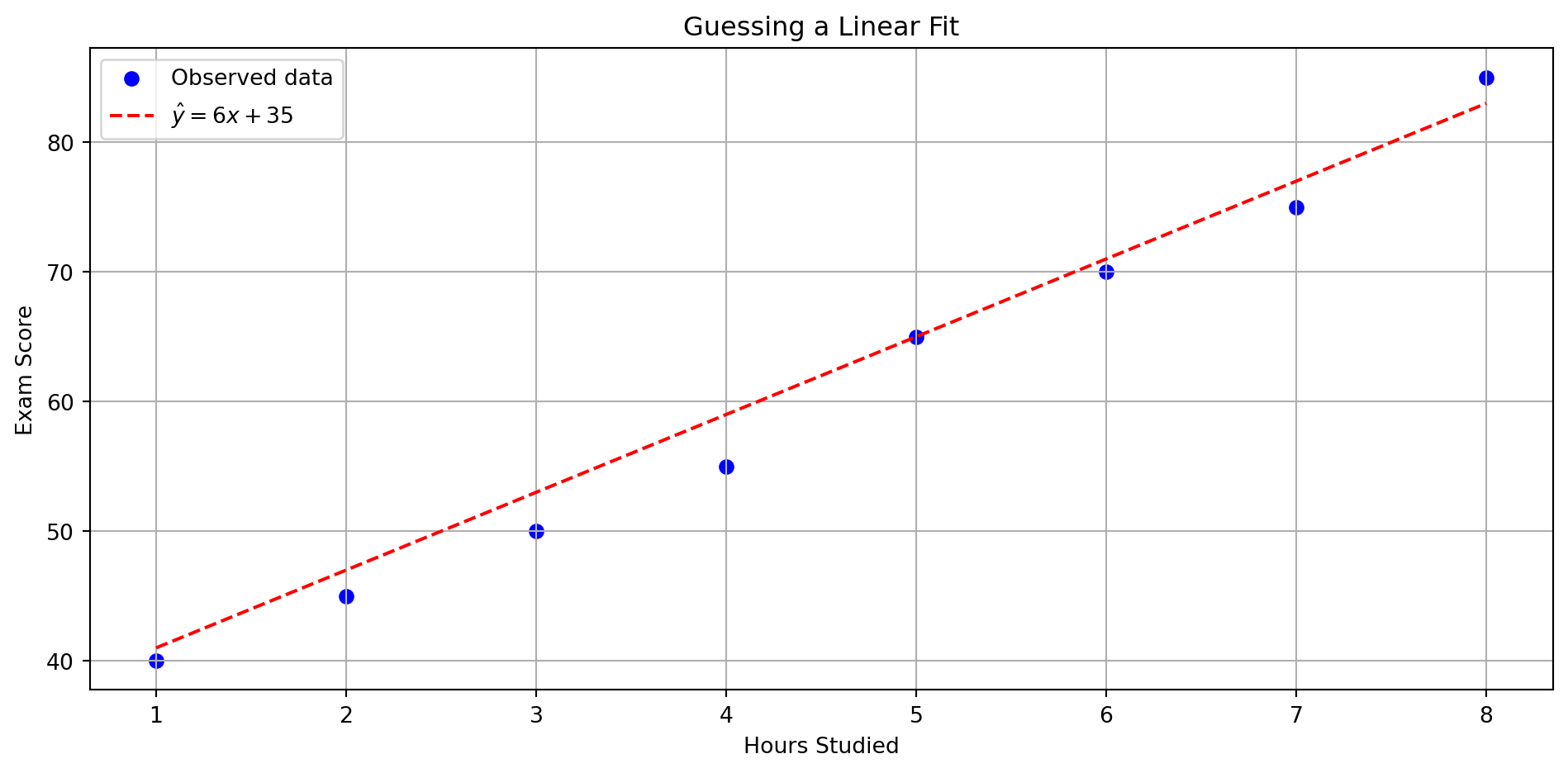
Recall: Linear Regression
Given a dataset of students’ study hours and exam scores, we used linear regression to predict the actual score.
- Input (x): Hours studied
- Output (y): Exam score
- Goal: Fit a line to predict score from hours
Fitting A Line
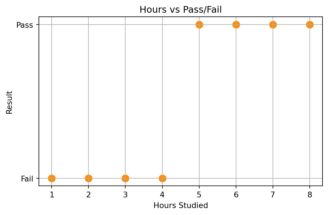
What If We Only Care About Pass/Fail?
In some applications, we don’t need the exact score — we just want to know:
Will the student pass the exam?
Let’s say:
- Score ≥ 60 → Pass (1)
- Score < 60 → Fail (0)
Now our goal becomes classification, not regression.
Reformulating Our Output
Let’s reframe our dataset:
Instead of predicting the actual score, we now assign a label:
- 1 = Pass (Score ≥ 60)
- 0 = Fail (Score < 60)
This gives us a new set of training labels:
\(y = [0, 0, 0, 0, 1, 1, 1, 1]\)
Visualization
What If We Still Use Linear Regression?
Suppose we treat the Pass/Fail labels (\(0\) or \(1\)) as numerical values and fit a linear regression model.
Let’s see what the model produces.
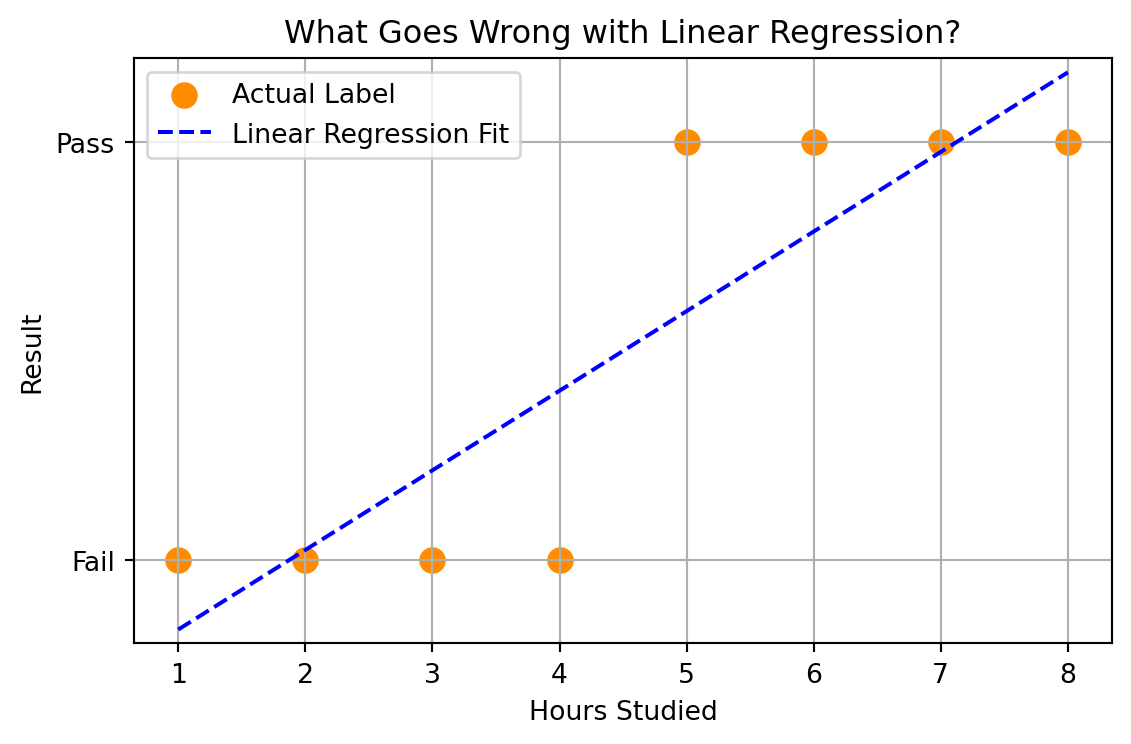
Why Linear Regression Does Not Work?
Linear regression tries to fit a best line to the numerical labels (0 and 1), but:
- It does not model probabilities
- The prediction can be < 0 or > 1
- There’s no guarantee that points on the same side of the line belong to the same class
This means it does not behave like a true classifier.
From Regression to Classification
In a classification problem:
- The goal is to assign an input \(x\) to one of several discrete categories (classes).
- In binary classification, there are only two possible labels, typically encoded as:
- 0 = Negative class (e.g., Fail)
- 1 = Positive class (e.g., Pass)
Unlike regression, we are not predicting a number, but a category.
Examples of Classification Problems
Many real-world problems require us to predict a category, not a number:
| Input | Prediction Goal | Type |
|---|---|---|
| Spam / Not Spam | Binary | |
| Tumor scan | Benign / Malignant | Binary |
| Image | Cat / Dog / Bird | Multiclass |
| Handwritten digit image | Digit (0–9) | Multiclass |
| Bank transaction | Fraud / Not Fraud | Binary |
| Hours studied | Pass / Fail | Binary |
| Sensor data from vehicle | Normal / Warning / Critical | Multiclass |
In classification, we care about which class an example belongs to — not the exact number.
Regression vs Classification
| Regression | Classification | |
|---|---|---|
| Output | Real-valued (e.g., exam score) | Class label (e.g., pass/fail) |
| Model output | A number in \((-\infty, \infty)\) | A class index or probability |
| Loss function | Squared loss, MAE, etc. | 0–1 loss, log loss, etc. |
| Example | Predict exam score | Predict pass or fail |
| Interpretation | “How much?” | “Which one?” |
Classification is often modeled probabilistically, especially in binary cases, where:
- The model outputs a number in [0, 1], interpreted as the probability of the positive class
- We apply a decision threshold (e.g., 0.5) to assign the final class
Setup
In ML, we observe:
- Input: \(\mathbf{x}_i\) (features)
- Output: \(y_i \in \{0, 1\}\)
Our goal: learn a model that predicts \[ \boxed{p(y = 1 \mid \mathbf{x})} \]
Why? Because that gives us:
- A classification decision
- A confidence score
From Linear Function to Classifier
We start with a linear function: \[ h(\mathbf{x}+) = \mathbf{w}^\top\mathbf{x}+b \]
Can we directly use \(h(\mathbf{x})\) as prediction?
- No — the output is a real number, not a valid class label.
- We need a decision rule to convert this into a classification.
A reasonable decision rule:
\[ \begin{aligned} &\hat{y} = 1 \quad \text{if } h(\mathbf{x}) \geq 0 \\ &\hat{y} = -1 \quad \text{otherwise} \end{aligned} \quad\Rightarrow\quad \hat{y} = \operatorname{sign}(\mathbf{w}^\top \mathbf{x}+b) \]
What does this define?
- A linear classifier.
- The decision boundary is the hyperplane: \[ \mathbf{w}^\top \mathbf{x} + b = 0 \]
- This separates the space into two half-spaces.
Simplifying with Data Augmentation
To simplify notation, we can augment the feature vector:
- Let \(\tilde{\mathbf{x}} = [1, \mathbf{x}^\top]^\top\)
- Let \(\tilde{\mathbf{w}} = [b, \mathbf{w}^\top]^\top\)
This lets us merge bias \(b\) into weights \(\mathbf{w}\).
What Are Log-Odds?
We define the odds of success as:
\[ \text{odds} = \frac{P(y=1 \mid x)}{P(y=0 \mid x)} = \frac{p}{1-p} \]
Then take the logarithm to get the log-odds (also called logit):
\[ \log\left(\frac{p}{1 - p}\right) = \text{linear in } x \]
The Decision Boundary (Log-Odds = 0)
We model the log-odds of class 1 vs class 0 as a linear function:
\[ \log \frac{p(y=1 \mid \mathbf{x})}{p(y=0 \mid \mathbf{x})} = \mathbf{w} ^\top \mathbf{x} \]
The decision boundary is where we are equally likely to choose either class:
\[ \log \frac{p(y=1 \mid \mathbf{x})}{p(y=0 \mid \mathbf{x})} = 0 \quad \Longrightarrow \quad \mathbf{w} ^\top \mathbf{x} = 0 \]
This is a linear boundary in the feature space, just like in linear regression!
But now, the output is interpreted probabilistically.
Solving for \(p(y=1 \mid \mathbf{x})\)
Recall: \[ \log \frac{p}{1 - p} = \mathbf{w} ^\top \mathbf{x} \]
Exponentiate both sides: \[ \frac{p}{1 - p} = \exp(\mathbf{w} ^\top \mathbf{x}) \]
Solve for \(p\): \[ \Rightarrow p = \frac{1}{1 + \exp(-\mathbf{w} ^\top \mathbf{x})} \]
This is the sigmoid function!
From Bernoulli to \(p(y \mid \mathbf{x})\)
Before: \(y_i \sim \text{Bernoulli}(p)\) with constant \(p\)
Now: \(y_i \sim \text{Bernoulli}(p_i)\) where \(p_i\) depends on \(\mathbf{x}_i\)
We model: \[ p(y_i = 1 \mid \mathbf{x}_i) = \sigma(\mathbf{w}^\top \mathbf{x}_i) \]
This is the core idea behind logistic regression:
- Turn input \(\mathbf{x}_i\) into a score
- Pass through sigmoid to get probability
In-Class Exercise
Recall the sigmoid function:
\[ \sigma(a) = \frac{1}{1 + e^{-a}} \]
Task: Derive \(\frac{d\sigma(a)}{da}\)
Hint:
- Use chain rule.
- Express your final answer in terms of \(\sigma(a)\).
Solution: Derivative of Sigmoid
Recall: \[ \sigma(a) = \frac{1}{1 + e^{-a}} \]
Take derivative:
\[ \begin{aligned} \frac{d\sigma(a)}{da} &= \frac{d}{da} \left( \frac{1}{1 + e^{-a}} \right) \\ &= \frac{e^{-a}}{(1 + e^{-a})^2} \\ &= \sigma(a) \cdot (1 - \sigma(a)) \end{aligned} \]
The sigmoid derivative is maximum at \(a = 0\) and symmetric about the origin.
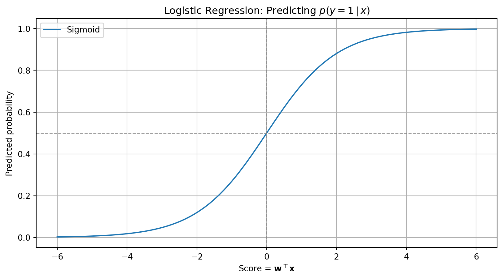
Visualization: Predicting \(p(y = 1 \mid x)\)
Logistic Regression via MLE
We define a probabilistic model for binary classification:
\[ p(y = 1 \mid \mathbf{x}) = \frac{1}{1 + \exp(-\mathbf{w}^\top \mathbf{x})} \]
Given a dataset \(\{(\mathbf{x}_i, y_i)\}_{i=1}^n\), and assuming i.i.d.:
\[ \mathcal{L}(\mathbf{w}) = \prod_{i=1}^n p(y_i \mid \mathbf{x}_i; \mathbf{w}) = \prod_{i=1}^n \left( \frac{1}{1 + \exp(-\mathbf{w}^\top \mathbf{x}_i)} \right)^{y_i} \left( 1 - \frac{1}{1 + \exp(-\mathbf{w}^\top \mathbf{x}_i)} \right)^{1 - y_i} \]
We want to maximize the likelihood \(\mathcal{L}(\mathbf{w})\).
Log-Likelihood: More Convenient
Take the log of the likelihood:
\[ \log \mathcal{L}(\mathbf{w}) = \sum_{i=1}^n \left[ y_i \log p(y_i = 1 \mid \mathbf{x}_i) + (1 - y_i) \log (1 - p(y_i = 1 \mid \mathbf{x}_i)) \right] \]
Plug in the sigmoid model:
\[ = \sum_{i=1}^n \left[ y_i \log \sigma(\mathbf{w}^\top \mathbf{x}_i) + (1 - y_i) \log (1 - \sigma(\mathbf{w}^\top \mathbf{x}_i)) \right] \]
This is the log-likelihood objective we maximize.
Logistic Regression as Loss Minimization
Define the log-loss (a.k.a. cross-entropy loss) per example:
\[ \ell(\hat{y}_i, y_i) = - y_i \log \hat{y}_i - (1 - y_i) \log (1 - \hat{y}_i) \]
The total loss:
\[ \mathcal{L}(\mathbf{w}) = \frac{1}{n} \sum_{i=1}^n \ell(\hat{y}_i, y_i) \]
This is exactly the negative log-likelihood!
MLE maximization = Log-loss minimization
Two Views, Same Objective
- Probabilistic View:
- Assume \(p(y \mid \mathbf{x})\) follows a Bernoulli distribution.
- Use MLE to find the best \(\mathbf{w}\).
- Optimization View:
- Define loss function based on how “wrong” the predictions are.
- Use log-loss (cross-entropy).
Both lead to the same training objective: \[ \arg \min_{\mathbf{w}} \sum_{i=1}^n \left[ - y_i \log \sigma(\mathbf{w}^\top \mathbf{x}_i) - (1 - y_i) \log (1 - \sigma(\mathbf{w}^\top \mathbf{x}_i)) \right] \]
Logistic regression is both statistically principled and computationally convenient.
Multiclass Logistic Regression
Why Multiclass?
Logistic regression models:
\[ P(y = 1 \mid \mathbf{x}) = \sigma(\mathbf{w}^\top \mathbf{x}) \]
Works well for binary classification (\(y \in \{0, 1\}\))
But what if we have more than two classes, say \(y \in \{0, 1, 2\}\)?
We need a new model that can handle multiclass probabilities.
What If We Have More Than Two Classes?
In binary classification:
\[ P(y = 1 \mid \mathbf{x}) = \sigma(\mathbf{w}^\top \mathbf{x}) \]
But what if \(y \in \{0, 1, 2, \dots, K-1\}\)?
How do we generalize logistic regression?
Softmax to Help!
Let’s model the log-odds of each class against a reference (e.g., class 0):
\[ \log \frac{P(y = k \mid \mathbf{x})}{P(y = 0 \mid \mathbf{x})} = \mathbf{w}_k^\top \mathbf{x}, \quad \text{for } k = 1, \dots, K - 1 \]
Rewriting:
\[ P(y = k \mid \mathbf{x}) = P(y = 0 \mid \mathbf{x}) \cdot e^{\mathbf{w}_k^\top \mathbf{x}} \]
Sum over all classes:
\[ 1 = \sum_{j=0}^{K-1} P(y = j \mid \mathbf{x}) = P(y = 0 \mid \mathbf{x}) \left(1 + \sum_{k=1}^{K-1} e^{\mathbf{w}_k^\top \mathbf{x}}\right) \]
Solve for \(P(y = 0 \mid \mathbf{x})\):
\[ P(y = 0 \mid \mathbf{x}) = \frac{1}{1 + \sum_{k=1}^{K-1} e^{\mathbf{w}_k^\top \mathbf{x}}} \]
Deriving the Softmax Function
Now plug back to get \(P(y = k \mid \mathbf{x})\):
For \(k = 0\): \[ P(y = 0 \mid \mathbf{x}) = \frac{1}{\sum_{j=0}^{K-1} e^{\mathbf{w}_j^\top \mathbf{x}}} \]
For \(k > 0\): \[ P(y = k \mid \mathbf{x}) = \frac{e^{\mathbf{w}_k^\top \mathbf{x}}}{\sum_{j=0}^{K-1} e^{\mathbf{w}_j^\top \mathbf{x}}} \]
Let’s define \(\mathbf{w}_0^\top \mathbf{x} = 0\) to simplify notation.
Then for all \(k\):
\[ P(y = k \mid \mathbf{x}) = \frac{e^{\mathbf{w}_k^\top \mathbf{x}}}{\sum_{j=0}^{K-1} e^{\mathbf{w}_j^\top \mathbf{x}}} \]
This is the softmax function
Softmax Generalizes Sigmoid
Binary case (\(K = 2\) classes):
The sigmoid function is: \[ \sigma(z) = \frac{1}{1 + e^{-z}} \]
This is equivalent to a 2-class softmax
In-Class Exercise
Let: \[ \hat{p}_k = \frac{e^{z_k}}{\sum_j e^{z_j}}, \quad \text{for } k = 1, \dots, K \]
Compute the partial derivative: \[ \frac{\partial \hat{p}_k}{\partial z_i} \]
- Case 1: \(k = i\)
- Case 2: \(k \neq i\)
Solution: Softmax Gradient (Jacobian)
We compute:
\[ \frac{\partial \hat{p}_k}{\partial z_i} = \begin{cases} \hat{p}_k (1 - \hat{p}_k) & \text{if } i = k \\ -\hat{p}_k \hat{p}_i & \text{if } i \neq k \end{cases} \]
This forms a matrix (Jacobian) of the form:
\[ J = \text{diag}(\hat{\mathbf{p}}) - \hat{\mathbf{p}} \hat{\mathbf{p}}^\top \]
Needed for computing gradients in softmax regression
Generalizing Binary Cross-Entropy
Binary Cross-Entropy:
\[ \mathcal{L} = -\left[ y \log \hat{y} + (1 - y) \log (1 - \hat{y}) \right] \]
Multiclass Cross-Entropy:
\[ \mathcal{L} = - \sum_{k=1}^K y_k \log \hat{p}_k \]
- \(y_k\) is a one-hot vector: only one \(y_k = 1\)
- \(\hat{p}_k\) is the output of the softmax layer
If \(K = 2\) and \(y = 1 \Rightarrow y_1 = 1, y_2 = 0\):
\[ \mathcal{L} = -\log \hat{p}_1 = -\log \sigma(z) \]
Multiclass CE reduces to binary CE when \(K = 2\)
Loss Function for Softmax Regression
Let \(y_i\) be the true label, \(\mathbf{x}_i\) the input, and \(K\) the number of classes.
Prediction probabilities: \[ \hat{p}_{ik} = \frac{e^{\mathbf{w}_k^\top \mathbf{x}_i}}{\sum_{j=1}^K e^{\mathbf{w}_j^\top \mathbf{x}_i}} \]
We use the multinomial cross-entropy loss:
\[ \mathcal{L} = - \sum_{i=1}^n \log \hat{p}_{i, y_i} \]
Same idea as binary log-loss, now over \(K\) classes
Training Softmax Regression
- Parameters: \(\mathbf{W} = [\mathbf{w}_1, \dots, \mathbf{w}_K]\)
- Optimize cross-entropy loss with gradient descent or SGD
Gradient for class \(k\):
\[ \nabla_{\mathbf{w}_k} \mathcal{L} = \sum_{i=1}^n \left( \hat{p}_{ik} - \mathbb{1}[y_i = k] \right) \mathbf{x}_i \]
Just like binary logistic regression, but with \(K\) sets of weights and softmax probabilities
Real-World Example: MNIST Digits
- MNIST is a famous dataset of handwritten digits.
- Each input is a \(28 \times 28\) grayscale image → flattened into a 784-dimensional vector.
- Labels: \(y \in \{0, 1, \dots, 9\}\)

A classic use case for multiclass logistic regression
One-Hot Encoding for Labels
In multiclass problems, labels \(y_i\) are integers like 3, 7, 9…
To compute gradients, we convert \(y_i\) into a one-hot vector:
Example for \(y_i = 3\) (10 classes):
\[ \mathbf{y}_i = [0, 0, 0, \color{blue}{1}, 0, 0, 0, 0, 0, 0] \]
Why?
- Compatible with cross-entropy loss
- Makes label differentiation easier during gradient computation