Logistic Regression
CISC 484/684 – Introduction to Machine Learning
Knowledge Check
KC 1

Maximum Likelihood Estimation
Motivation: Yes or No?
Suppose we’re predicting binary outcomes:
- Will the student pass the course? ✅ / ❌
- Will a customer click the ad?
- Is the email spam?
These are all binary classification problems.
The outcome is either 1 (success) or 0 (failure).
So how do we model this?
Bernoulli Intuition
\(\Pr(X = 1) = \mu\)
\(\Pr(X = 0) = 1 - \mu\)
So the PMF becomes:
- If \(x = 1\): \(\mu\)
- If \(x = 0\): \(1 - \mu\)
Very compact form: \[ \Pr(x) = \mu^x (1 - \mu)^{1 - x} \]
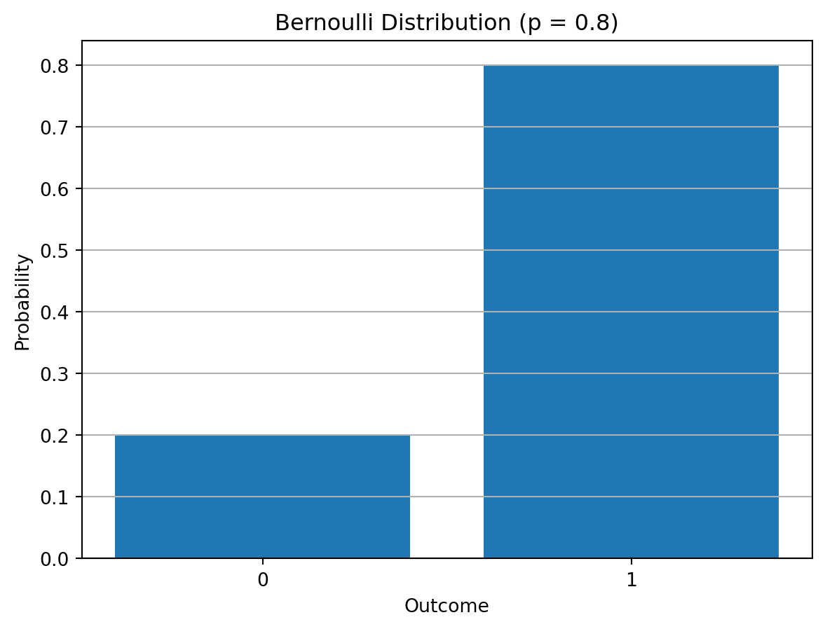
Bernoulli Distribution
The Bernoulli distribution models a single binary outcome: \[ x \in \{0, 1\} \]
It has one parameter: \(\mu \in [0, 1]\), the probability of success (\(x = 1\))
The probability mass function (PMF) is: \[ \Pr(X = x) = \mu^x (1 - \mu)^{1 - x}, \quad \text{for } x \in \{0, 1\} \]
This compact form covers both cases:
- \(x = 1\): \(\Pr(1) = \mu\)
- \(x = 0\): \(\Pr(0) = 1 - \mu\)
This will be useful when we do MLE.
Visualization
Flip Coins
- A single coin toss produces \(H\) or \(T\)
- Let’s try playing this game:
- Toss once: \(H\)
- Toss twice: \(HH\)
- Toss 1000 times: \(HHH\cdots H\) (all heads)
- Hmm… maybe the coin is not fair?
We use a parameter \(\mu \in [0, 1]\) to express the fairness of a coin.
A perfectly fair coin has \(\mu = 0.5\).
Problem Setup
For convenience, we encode \(H\) as 1 and \(T\) as 0
Define a random variable \(X \in \{0, 1\}\)
Then: \[ \Pr(X = 1; \mu) = \mu \]
For simplicity, we write \(p(x)\) or \(p(x; \mu)\) instead of \(\Pr(X = x; \mu)\)
The parameter \(\mu \in [0, 1]\) specifies the bias of the coin
Fair coin: \(\mu = \frac{1}{2}\)
Probability vs. Likelihood
These two are closely related, but not the same.
The difference is what is fixed and what is being varied.
| Concept | Probability | Likelihood |
|---|---|---|
| Fixed | Parameters (e.g., \(\mu\)) | Data (e.g., \(x_1, \dots, x_n\)) |
| Varies | Outcome (data) | Parameters |
| Usage | Sampling, prediction | Inference, estimation (MLE!) |
Probability: Predicting the Future
If I tell you:
“This is a fair coin: \(\mu = 0.5\)”
Then you ask:
“What’s the probability of getting \(HHH\)?”
We compute: \[ \Pr(HHH \mid \mu = 0.5) = (0.5)^3 = 0.125 \]
You know the model. You’re predicting data.
Likelihood: Explaining the Past
You say:
“I tossed a coin 3 times and got \(HHH\).”
Then you ask:
“What’s the most likely value of \(\mu\) that explains this?”
We evaluate: \[ L(\mu \mid \text{data}) = \mu^3 \]
- Likelihood is a function of \(\mu\)
- We’re saying: “How well does each \(\mu\) explain what we already observed?”
Side-by-side: Same formula, different roles
- For Bernoulli: \(\Pr(x ; \mu) = \mu^x (1 - \mu)^{1 - x}\)
Probability
- \(\mu\) is fixed
- \(x\) is random
- Used to predict new outcomes
Likelihood
- \(x\) is fixed
- \(\mu\) varies
- Used to estimate parameters (MLE)
Visual Intuition
Imagine you observe \(x = [1, 1, 1, 0, 1]\)
Probability: “If I assume \(\mu = 0.6\), how likely is this data?”
Likelihood: “Given this data, which \(\mu\) makes it most likely?”
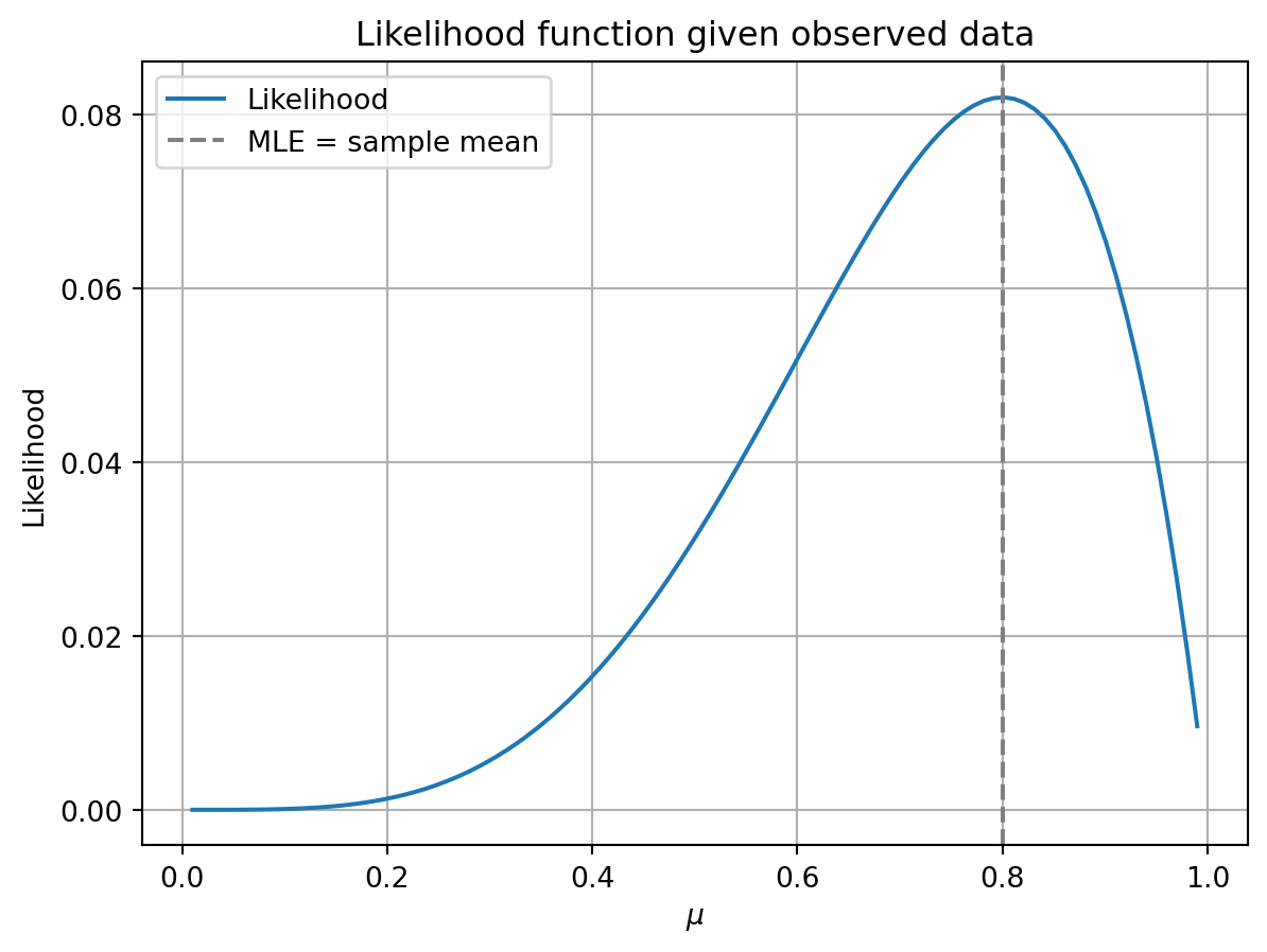
MLE for Bernoulli
Likelihood of an i.i.d. sample \(\mathbf{X} = [x_1, \dots, x_n]\): \[ L(\mu) = \Pr(\mathbf{X}; \mu) = \prod_{i=1}^n \mu^{x_i}(1 - \mu)^{1 - x_i} \]
Log-likelihood: \[ \ell(\mu) = \log L(\mu) = \sum_{i=1}^n \left[ x_i \log \mu + (1 - x_i) \log (1 - \mu) \right] \]
Because \(\log\) is monotonic: \[ \arg\max_\mu \, L(\mu) = \arg\max_\mu \, \log L(\mu) \]
Question: Why do we use the log-likelihood?
ML for Bernoulli
To find the MLE, we set the derivative to zero:
\[ \begin{aligned} \frac{d}{d\mu} \log L(\mu) &= \frac{1}{\mu} \sum_{i=1}^n x_i - \frac{1}{1 - \mu} \sum_{i=1}^n (1 - x_i) = 0 \\ \Rightarrow \frac{1 - \mu}{\mu} &= \frac{n - \sum x_i}{\sum x_i} \\ \Rightarrow \widehat{\mu}_{\text{ML}} &= \frac{1}{n} \sum_{i=1}^n x_i \end{aligned} \]
- The MLE is simply the fraction of heads in your data: \[ \boxed{\widehat{\mu}_{\text{ML}} = \text{average of } x_i} \]
What Might Be the Problem?
MLE isn’t always reliable with small samples:
If we toss a coin twice and get \(HT\), then \(\widehat{\mu}_{\text{ML}} = 0.5\)
→ Is this enough to say the coin is fair?If we toss it only once:
- One head → \(\widehat{\mu}_{\text{ML}} = 1\)
- One tail → \(\widehat{\mu}_{\text{ML}} = 0\)
From Regression to Classification
Our Goal: Predict Outcomes Given Features
We’re not just flipping biased coins anymore.
In ML, we observe:
- Input: \(\mathbf{x}_i\) (features)
- Output: \(y_i \in \{0, 1\}\)
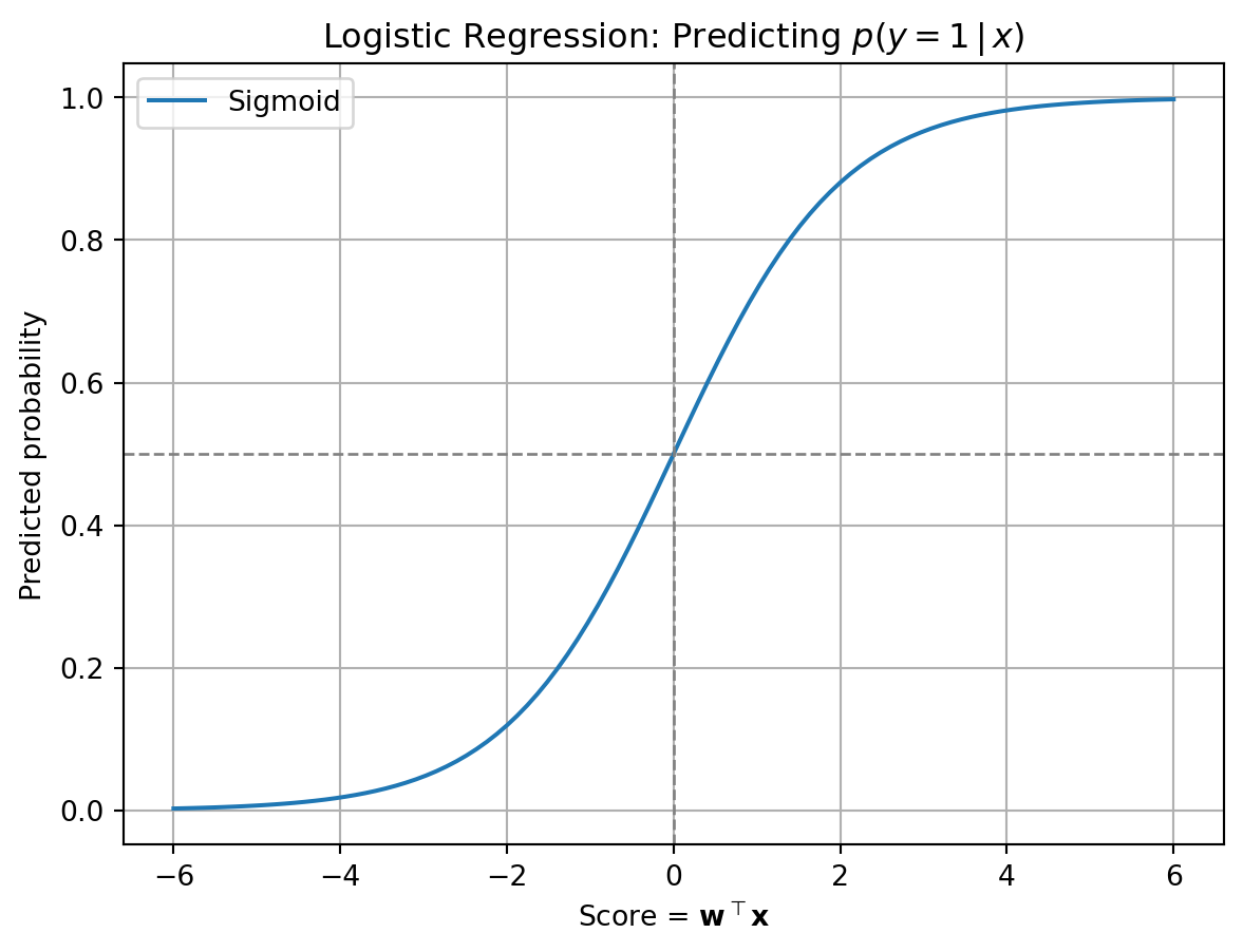
Our goal: learn a model that predicts \[ \boxed{p(y = 1 \mid \mathbf{x})} \]
Why? Because that gives us:
- A classification decision
- A confidence score
From Bernoulli to \(p(y \mid \mathbf{x})\)
Before: \(y_i \sim \text{Bernoulli}(p)\) with constant \(p\)
Now: \(y_i \sim \text{Bernoulli}(p_i)\) where \(p_i\) depends on \(\mathbf{x}_i\)
We model: \[ p(y_i = 1 \mid \mathbf{x}_i) = \sigma(\mathbf{w}^\top \mathbf{x}_i) \]
This is the core idea behind logistic regression:
- Turn input \(\mathbf{x}_i\) into a score
- Pass through sigmoid to get probability
Visualization: Predicting \(p(y = 1 \mid x)\)