Optimization Basics
CISC 484/684 – Introduction to Machine Learning
Sihan Wei
June 24, 2025
Measuring Size: \(L_p\) Norms
- A norm is a way to measure the size or length of a vector
- The most common family of norms are the \(L_p\) norms:
\[ \|\mathbf{x}\|_p = \left( \sum_{i=1}^n |x_i|^p \right)^{1/p} \]
- Depending on \(p\), the norm behaves differently.
Examples of \(L_p\) Norms
- \(L_1\) norm (Manhattan norm): \(\|\mathbf{x}\|_1 = \sum_i |x_i|\)
- “City block” distance
- \(L_2\) norm (Euclidean norm): \(\|\mathbf{x}\|_2 = \sqrt{\sum_i x_i^2}\)
- Straight-line distance
- \(L_\infty\) norm (Max norm): \(\|\mathbf{x}\|_\infty = \max_i |x_i|\)
- Just the biggest coordinate!
Why Do We Care?
- Norms are used to:
- Measure distance between vectors
- Penalize model complexity (e.g., in regularization)
- Define constraints in optimization
- In ML, you’ll often see:
- \(\|\mathbf{w}\|_2^2\) (Ridge regularization)
- \(\|\mathbf{w}\|_1\) (Lasso sparsity)
Summary
- The \(L_p\) norm generalizes “length” for different values of \(p\)
- \(L_2\) is most common (Euclidean)
- \(L_1\) is useful when we want sparsity
- Norms will appear everywhere: loss functions, constraints, gradients
Recall
For a linear regression problem, we have the closed-form solution:
\[\mathbf{w}=\left(\mathbf{X}^T \mathbf{X}\right)^{-1} \mathbf{X}^T \mathbf{y}\]
This is awesome, but:
- What if we only see one \((x_i, y_i)\) at a time?
- What if we have too much data to compute \((X^\top X)^{-1}\)?
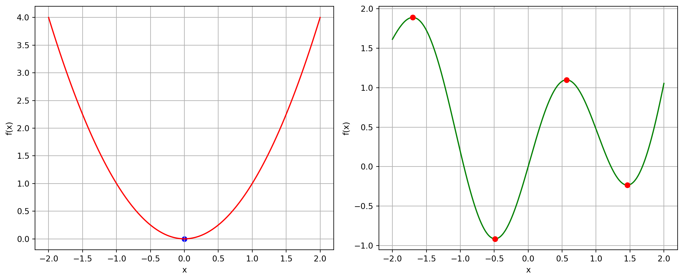
Convexity
- “The maximum is when the gradient is equal to 0”
- Is that true?
Convex Sets
\(A\) set \(S\) is convex if the line segment between any two points of S lies in S . That is, if for any \(x, y \in S\) and any \(\lambda \in[0,1]\) we have
\[ \lambda x+(1-\lambda) y \in S \]
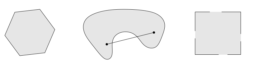
- Left: convex set
- Middle: non-convex set
- Right: non-convex set
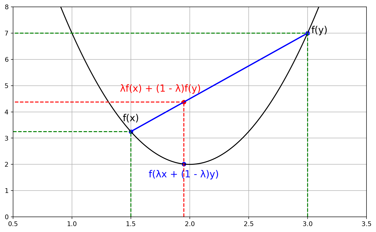
Convex Functions
- A function \(f: R^d \rightarrow R\) is convex if (i) \(\operatorname{dom}(f)\) is a convex set and (ii) \(\forall x, y \in \operatorname{dom}(f)\) and \(\lambda \in[0,1]\) we have
\[ f(\lambda x+(1-\lambda) y) \leq \lambda f(x)+(1-\lambda) f(y) \]
More intuitively, the line segment between any two points on its graph lies above the graph itself!
Benefits of convex functions: Every local minimum is a global minimum!
Convex Functions
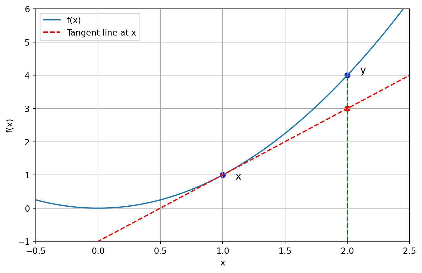
First-order condition
- Suppose that \(\operatorname{dom}(f)\) is open and that \(f\) is differentiable. Then \(f\) is convex if and only if \(\operatorname{dom}(f)\) is convex and for all \(x, y \in \operatorname{dom}(f)\) the following holds:
\[ f(y) \geq f(x)+\nabla f(x)^{\top}(y-x) \]
- Remark: The graph of the affine function \(f(x)+\) \(\nabla f(w)^{\top}(y-x)\) is a tangent hyperplane to the graph of \(f\) at ( \(x, f(x)\) ).
- That is, graph of function \(f\) is above all of its tangent hyperplanes.
First-order Condition
Examples of Convex Functions
Linear function: \(f(x)=a^{\top} x\)
- Affine function: \(f(x)=a^{\top}+b\)
- Exponential function: \(f(x)=e^{a x}\)
- Quadratic with \(a>0: f(x)=a x^2\)
- Norms on \(R^d: f(x)=\|x\|_2\)
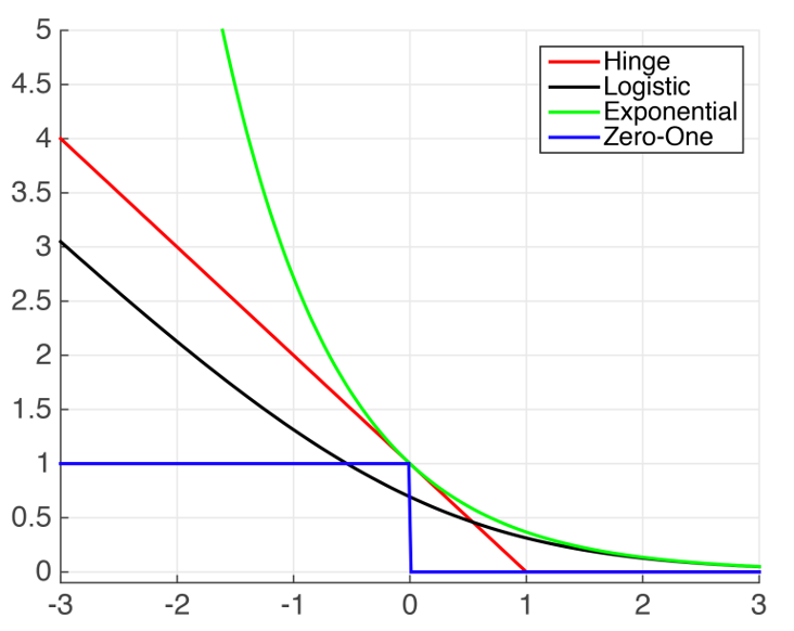
Loss functions
0-1 loss is ideal but hard to optimize!
- Non-convexity: there may be many local minima, makes it difficult for an optimization algorithm to find the best solution (global minimum).
- Discontinuity: any small change in the model parameters could lead to sudden jumps in the loss value, makes gradient-based algorithm impossible to use.
- No useful gradient information: the gradient is either 0 or undefined, and hence optimization algorithms cannot make informed updates.
Convex Surrogate Losses
- Hinge loss (in SVM): \(\ell_{\text{hin}}=\max\{0,1-z\}\)
- Logistic loss (in logistic regression): \(\ell_{\text{log}}=\log(1+\exp(-z))\)
- Exponential loss (in AdaBoost): \(\ell_{\text{exp}}=\exp(-z)\)
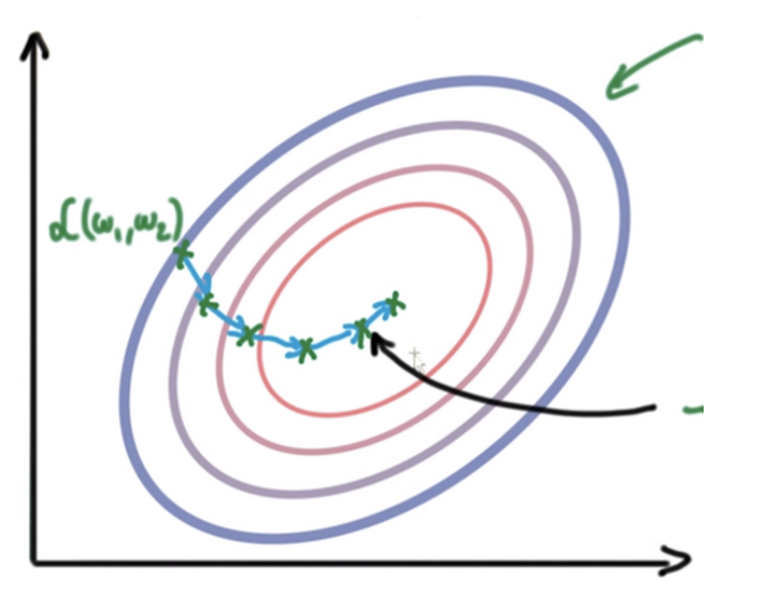
Gradient Descent: What Are We Trying to Do?
- We want to minimize a loss function.
- Imagine we’re trying to find the lowest point in a valley.
Going Downhill
Think of the loss surface as a hilly terrain.
You’re standing somewhere on the surface.
How do you move downhill toward the minimum?
You need two things:
- A direction (where to go)
- A step size (how far to go)
In machine learning, this is gradient descent!
What is the Gradient?
The gradient tells you the direction of steepest ascent
⟶ So to minimize, we go in the opposite directionMathematically: \[ \mathbf{w}_{t+1} = \mathbf{w}_t - \eta \nabla L(\mathbf{w}_t) \]
Where:
- \(\nabla L(\mathbf{w}_t)\) is the gradient of the loss
- \(\eta\) is the step size (aka learning rate)
Gradient Based Optimization
Our goal is to minimize the objective function
\[ \min _w f(w)=\frac{1}{n} \sum_{i=1}^n f_i(w) \]
Batch optimization
\[ w^{t+1}=w^t-\gamma_t \nabla f\left(w^t\right)=w^t-\gamma_t \frac{1}{n} \sum_{i=1}^n f_i\left(w^t\right) \]
Combine all derivatives into a single update
Gradient Based Optimization
- Pro
- Use all available information to update parameters
- Con
- Slow: must consider every data point
- How different is an update with n-1 vs. n examples?
GD for Linear Regression
The squared loss function for the entire dataset is
\[ f(\mathbf{w})=\frac{1}{2 n} \sum_{i=1}^n\left(\mathbf{w}^{\top} \mathbf{x}_i-y_i\right)^2=\frac{1}{2 n}\|\mathbf{X} \mathbf{w}-\mathbf{Y}\|_2^2 \]
The gradient is
\[ \nabla f(\mathbf{w})=\frac{1}{n} \sum_{i=1}^n\left(\mathbf{w}^{\top} \mathbf{x}_i-y_i\right) \mathbf{x}_i=\frac{1}{n} \mathbf{X}^{\top}(\mathbf{X} \mathbf{w}-\mathbf{Y}) \]
For \(t\)-th iteration, we update
\[ \mathbf{w}^{t+1}=\mathbf{w}^t-\gamma_t \frac{1}{n} \sum_{i=1}^n\left(\mathbf{w}^{t^{\top}} \mathbf{x}_i-y_i\right) \mathbf{x}_i \]
and the matrix version is
\[ \mathbf{w}^{t+1}=\mathbf{w}^t-\gamma_t \frac{1}{n} \mathbf{X}^{\top}\left(\mathbf{X} \mathbf{w}^t-\mathbf{Y}\right) \]
Gradient Descent
A typical GD algorithm
- We show pseudocode for gradient descent
- Initialize \(w\) and a threshold parameter \(\epsilon\) (e.g. 1e-3)
- Repeat until convergence
- Choose learning rate \(\gamma_t\) (could be a constant)
- Compute the full gradient \(\nabla f(w)\)
- Update parameter \(w^{t+1}=w^t-\gamma_t \nabla f\left(w^t\right)\)
- If \(\left\|w^{t+1}-w^t\right\| \leq \epsilon\), exit the loop
Stochastic Gradient Descent
- Update rule: \(w^{t+1}=\mathrm{w}^{\mathrm{t}}-\gamma_t \nabla f_i\left(w^t\right)\)
- \(\nabla f_i(x)\) is an unbiased estimator of the true gradient \(\nabla f(x)\). That is, \(\mathbb{E}\left[\nabla f_i(x)\right]=\nabla f(x)\)
- Updates parameters after each example
- Pro– Fast: each update considers a single example, improves parameters faster
- Con– Noisy updates: Each update based on very little information
Stochastic Gradient Descent
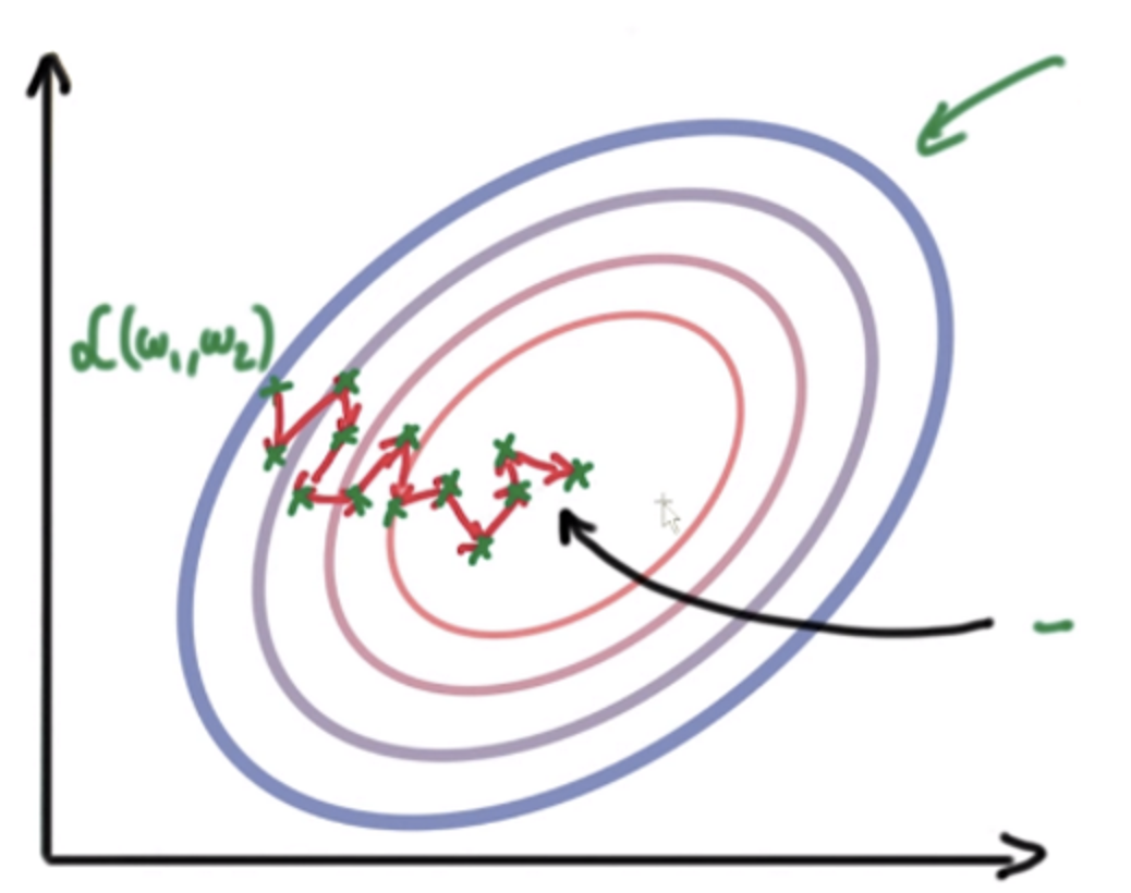
Uniform Single-element Sampling SGD
At each iteration, we do the following steps:
- Uniformly at random select \(i \in[n]\left(p_i=\frac{1}{n}\right)\)
- Compute \(\nabla f_i\left(w^t\right)\)
- Update \(w^{t+1}=w^t-\gamma_t \nabla f_i\left(w^t\right)\)
- Note there are many other sampling methods!
SGD for Linear Regression
Recall
\[ f(\mathbf{w})=\frac{1}{n} \sum_{i=1}^n f_i(\mathbf{w})=\frac{1}{2 n} \sum_{i=1}^n\left(\mathbf{w}^{\top} \mathbf{x}_i-y_i\right)^2 \]
Hence, the squared loss for a single data sample ( \(\mathbf{x}_i, y_i\) ) is
\[ f_i(\mathbf{w})=\frac{1}{2}\left(\mathbf{w}^{\top} \mathbf{x}_i-y_i\right)^2 \]
The gradient of \(f_i\) is
\[ \nabla f_i(\mathbf{w})=\left(\mathbf{w}^{\top} \mathbf{x}_i-y_i\right) \mathbf{x}_i \]
For \(t\)-th iteration, we update
\[ \mathbf{w}^{t+1}=\mathbf{w}^t-\gamma_t\left(\mathbf{w}^{t^{\top}} \mathbf{x}_i-y_i\right) \mathbf{x}_i \]