Linear Regression
CISC 484/684 – Introduction to Machine Learning
Sihan Wei
June 17, 2025
Announcements
- HW 1 Released
- Due next Tuesday at 11:59 PM
- Let me know if you have any questions
- Due next Tuesday at 11:59 PM
Quick Recap
- ML Setup
- Hypothesis class and model complexity
- Loss functions
- 0–1 loss
- Squared loss
- Empirical risk vs generalization risk
- Underfitting vs overfitting
- Bias–variance tradeoff
Appears in Homework — please review!
Understand the error decomposition:
\[ \mathbb{E}[(\hat{y} - y)^2] = \text{Bias}^2 + \text{Variance} + \text{Noise} \]
No derivation required, but be sure you know why the cross-term is zero.
Why Linear Regression?
- One of the oldest and simplest ML models.
- Often surprisingly effective with good features.
- Foundation for more advanced models (logistic regression, neural nets).
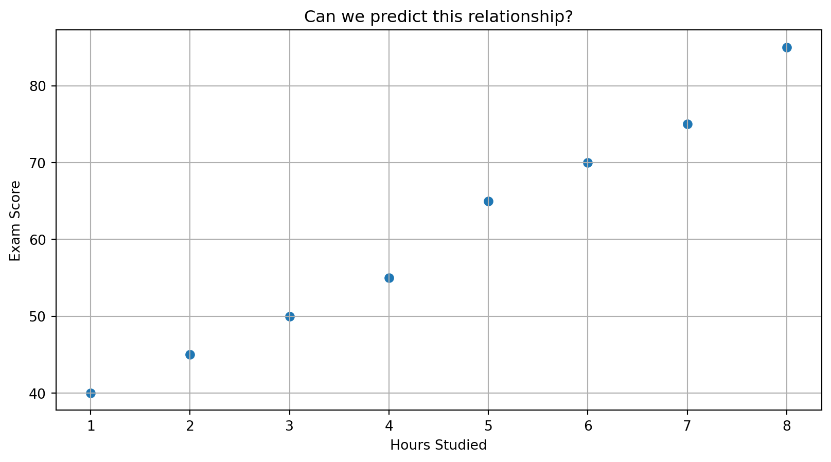
Predicting Exam Scores
Can We Fit a Line?
We want to predict score from hours studied:
Find a rule of the form:
\(\hat{y} = w x + b\)
- \(\hat{y}\) is the predicted exam score
- \(x\) is the number of study hours
- \(w\) is the slope (how much score increases per hour)
- \(b\) is the intercept (score when \(x = 0\))
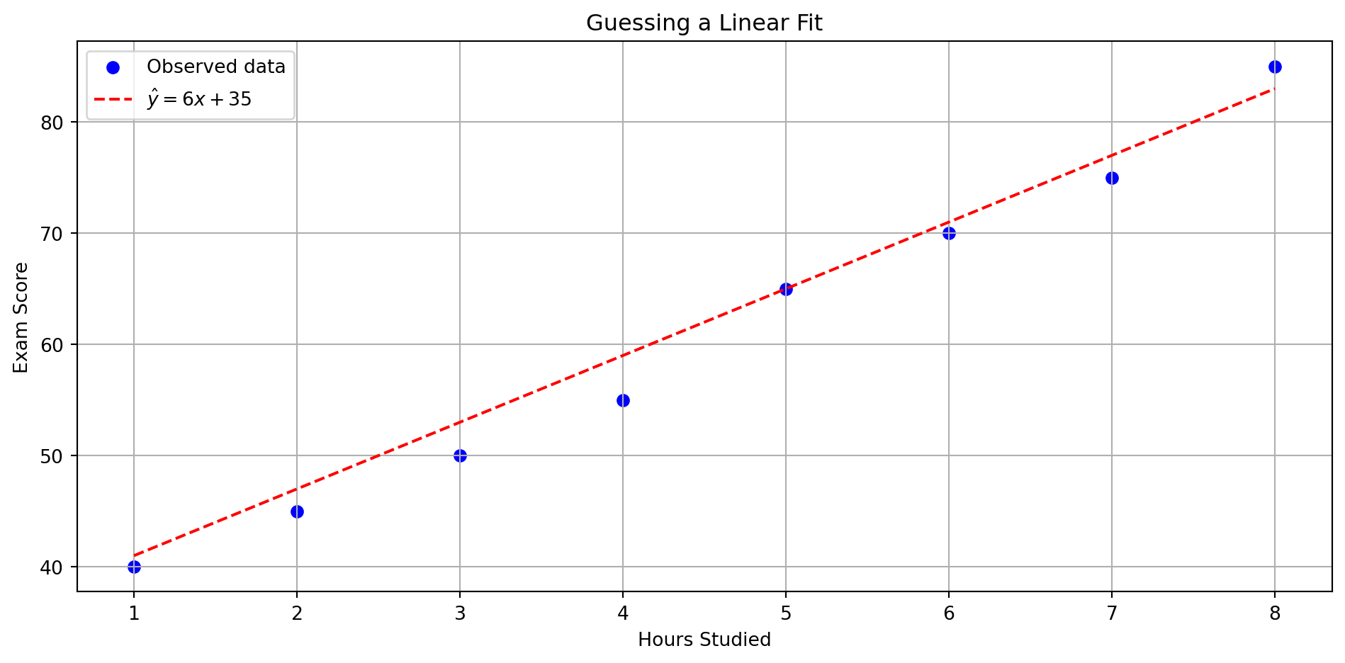
Let’s eyeball a possible line…
Guessing A Line
Checkpoint
We guessed:
\(\hat{y} = 6x + 35\)
- What is the predicted score for 6 hours of study?
- What is the error if the actual score was 70?
Solution
- \(\hat{y} = 6 \cdot 6 + 35 = 71\)
- Error = \(70 - 71 = -1\)
From Data to Model
We want to predict exam score based on hours studied.
- Input: \(x\) = hours of study
- Output: \(y\) = exam score
- Goal: Find a simple function that maps \(x \rightarrow y\)
Let’s try a linear model:
\[ \hat{y} = wx + b \]
- \(\hat{y}\) is the predicted score
- \(w\) is the slope: how much the score increases per hour
- \(b\) is the intercept: base score when \(x = 0\)
This is the linear regression model — our job is to find the best values of \(w\) and \(b\) from data.
Formal Definition
We assume a linear relationship between input \(x\) and output \(y\):
\[ \hat{y} = wx + b \]
In this model:
- \(x \in \mathbb{R}\): the input (e.g., hours studied)
- \(y \in \mathbb{R}\): the true output (e.g., exam score)
- \(\hat{y} \in \mathbb{R}\): the predicted output
- \(w, b \in \mathbb{R}\): model parameters (slope and intercept)
Also known as least squares regression.
More generally, for multidimensional input \(\mathbf{x} \in \mathbb{R}^d\):
\[ \hat{y} = \mathbf{w}^\top \mathbf{x} + b \]
Where:
- \(\mathbf{x} = [x_1, \dots, x_d]^\top\): feature vector
- \(\mathbf{w} = [w_1, \dots, w_d]^\top\): weights
- \(b\): bias term
We aim to learn \(w\) and \(b\) from data such that \(\hat{y}\) closely approximates \(y\).
What Makes a Good Fit?
Our model predicts \(\hat{y}\), but real \(y\) may differ.
Example:
| Hours (\(x\)) | True (\(y\)) | Predicted (\(\hat{y}\)) | Error (\(\hat{y} - y\)) |
|---|---|---|---|
| 4 | 55 | 60 | \(+5\) |
| 6 | 70 | 71 | \(+1\) |
| 8 | 85 | 83 | \(-2\) |
- How do we quantify how wrong our predictions are?
- How do we train the model to be better?
Which Line Fits Better?
Let’s compare two candidate lines:
- Fit A: \(\hat{y}_1 = 6x + 35\)
- Fit B: \(\hat{y}_2 = 4x + 45\)
Both are straight. But are they equally good?
Which line better explains the observed data?
Two linear models
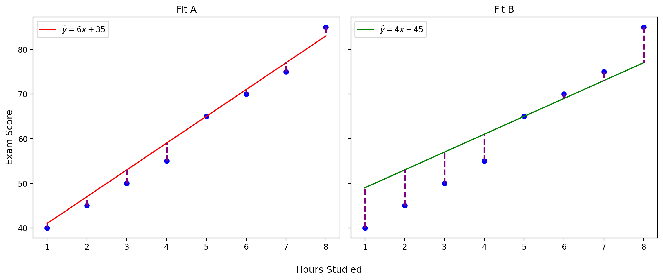
How Do We Decide Which Line Is Better?
Both lines are straight.
Both make some predictions.
But one line’s predictions are consistently closer to the actual data.
We need a way to quantify the total error between predicted and observed values.
That’s where loss functions come in.
Squared Loss
\[ \ell_{\text{sq}}(\hat{y}, y) = (\hat{y} - y)^2 \]
- Penalizes large errors more heavily
- Always non-negative
- Smooth and differentiable
Mean Squared Error (MSE)
Given \(n\) data points \((x_i, y_i)\):
\[ \text{MSE}(w, b) = \frac{1}{n} \sum_{i=1}^{n} \left( \hat{y}_i - y_i \right)^2 = \frac{1}{n} \sum_{i=1}^{n} \left( w^\top x_i + b - y_i \right)^2 \]
- Average squared loss over the dataset
- This is the objective function we want to minimize
We’ll soon see: this comes from a probabilistic assumption.
From Deterministic to Probabilistic Model
So far, we’ve assumed a deterministic prediction:
\[ \hat{y} = wx + b \]
But in reality, outputs contain random noise — exam scores can vary even with the same study hours.
We model this uncertainty as:
\[ y = \hat{y} + \varepsilon = wx + b + \varepsilon \]
Assume:
\[ \varepsilon \sim \mathcal{N}(0, \sigma^2) \]
Then the output \(y\) is normally distributed around the predicted value:
\[ y \sim \mathcal{N}(wx + b, \sigma^2) \]
Recap: Gaussian (Normal) Distribution
A Gaussian (normal) distribution looks like a bell curve:
\[ \mathcal{N}(\mu, \sigma^2) = \frac{1}{\sqrt{2\pi \sigma^2}} \exp\left( -\frac{(y - \mu)^2}{2\sigma^2} \right) \]
- \(\mu\): the mean (center of the curve)
- \(\sigma^2\): the variance (spread of the curve)
Most real-world measurements (e.g., test scores, noise) are approximately Gaussian!
Visualizing Gaussian Distributions
- 1D: Bell curve
- 2D: Bell surface
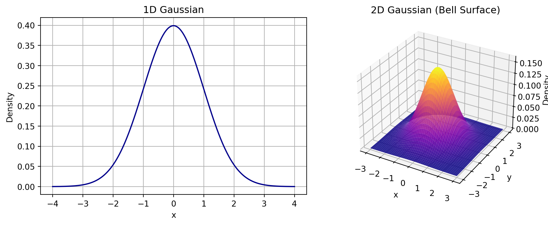
More Visualizations
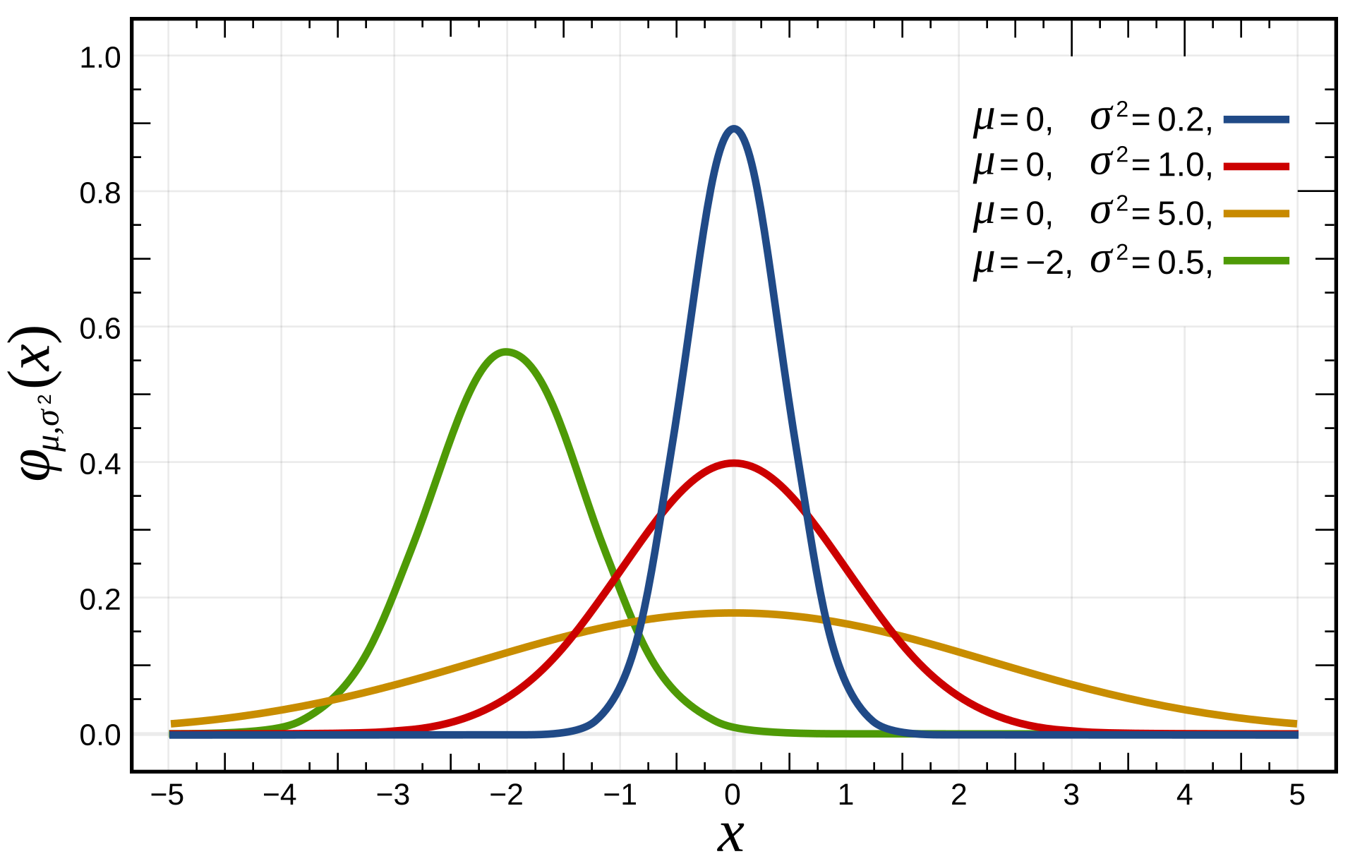
Image source: Wikipedia
Probabilistic Interpretation: Likelihood
Given a dataset \(\{(x_i, y_i)\}_{i=1}^n\), the likelihood of the parameters \((w, b)\) is:
\[ \mathcal{L}(w, b) = \prod_{i=1}^n P(y_i \mid x_i; w, b) \]
Each \(y_i\) is assumed drawn from:
\[ y_i \sim \mathcal{N}(wx_i + b, \sigma^2) \]
So:
\[ P(y_i \mid x_i; w, b) = \frac{1}{\sqrt{2\pi \sigma^2}} \exp\left( -\frac{(y_i - wx_i - b)^2}{2\sigma^2} \right) \]
Taking logs:
\[ \log \mathcal{L}(w, b) = -\frac{1}{2\sigma^2} \sum_{i=1}^n (y_i - wx_i - b)^2 + \text{const} \]
Maximum Likelihood = Least Squares
Maximizing log-likelihood is the same as:
\[ \arg\max_{w,b} \log \mathcal{L}(w, b) \quad \Longleftrightarrow \quad \arg\min_{w,b} \sum_{i=1}^n (y_i - wx_i - b)^2 \]
This is mean squared error (MSE) minimization.
So, when we assume Gaussian noise, linear regression with MSE loss is performing maximum likelihood estimation (MLE)!
Linear Regression in Matrix Form
We now move to multivariate linear regression:
\[ \hat{y} = \mathbf{w}^\top \mathbf{x} + b \]
To simplify notation, we fold the bias into the weights:
Augment the input:
\[ \tilde{\mathbf{x}} = \begin{bmatrix} x_1 \\ x_2 \\ \vdots \\ x_d \\ 1 \end{bmatrix} \quad \tilde{\mathbf{w}} = \begin{bmatrix} w_1 \\ w_2 \\ \vdots \\ w_d \\ b \end{bmatrix} \]
Then:
\[ \hat{y} = \tilde{\mathbf{w}}^\top \tilde{\mathbf{x}} \]
Now suppose we have \(n\) examples.
Let:
- \(X \in \mathbb{R}^{n \times (d+1)}\): input matrix (each row = \(\tilde{\mathbf{x}}_i\))
- \(\mathbf{y} \in \mathbb{R}^n\): vector of true labels
- \(\hat{\mathbf{y}} = X \tilde{\mathbf{w}}\): predicted outputs
Benefits of Vectorizing your code?
Computational Efficiency: Matrix operations can be highly optimized by modern CPUs and GPUs, taking advantage of vectorized operations and parallel processing.
Simplicity: Using matrix formulations makes your code closely match their math formulation. You can write more readable code.
Scalability: Matrix operations allow for more scalable and flexible algorithm implementations.
MSE Loss in Matrix Form
Our goal is to minimize Mean Squared Error:
\[ \mathcal{L}(\tilde{\mathbf{w}}) = \frac{1}{2}\| X \tilde{\mathbf{w}} - \mathbf{y} \|^2 = \frac{1}{2}(X \tilde{\mathbf{w}} - \mathbf{y})^\top (X \tilde{\mathbf{w}} - \mathbf{y}) \]
This is a convex quadratic function of \(\tilde{\mathbf{w}}\).
To find the optimal \(\tilde{\mathbf{w}}\), take the gradient:
\[ \nabla_{\tilde{\mathbf{w}}} \mathcal{L} = X^\top (X \tilde{\mathbf{w}} - \mathbf{y}) \]
Set the gradient to zero:
\[ X^\top X \tilde{\mathbf{w}} = X^\top \mathbf{y} \]
Closed-Form Solution for Linear Regression
From:
\[ X^\top X \tilde{\mathbf{w}} = X^\top \mathbf{y} \]
Assuming \(X^\top X\) is invertible:
\[ \tilde{\mathbf{w}} = (X^\top X)^{-1} X^\top \mathbf{y} \]
This is the maximum likelihood estimator under Gaussian noise,
and also the solution to the least squares problem.
- No optimization algorithm needed
- In practice: might regularize or use gradient methods instead.
Ridge Regression (L2 Regularization)
Add an \(\ell_2\) penalty to the loss:
\[ \mathcal{L}_{\text{ridge}}(\mathbf{w}) = \sum_{i=1}^n (y_i - \mathbf{w}^\top \mathbf{x}_i)^2 + \lambda \|\mathbf{w}\|_2^2 \]
- \(\lambda \ge 0\): regularization strength
- Larger \(\lambda\): encourages smaller weights
- Prevents overfitting by shrinking model complexity
Closed-form solution:
\[ \mathbf{w}_{\text{ridge}} = (X^\top X + \lambda I)^{-1} X^\top \mathbf{y} \]
Always invertible if \(\lambda > 0\)
Lasso Regression (L1 Regularization)
Use \(\ell_1\) penalty instead:
\[ \mathcal{L}_{\text{lasso}}(\mathbf{w}) = \sum_{i=1}^n (y_i - \mathbf{w}^\top \mathbf{x}_i)^2 + \lambda \|\mathbf{w}\|_1 \]
- Encourages sparsity: many weights become exactly 0
- Helps with feature selection
- No closed-form solution — solved via optimization
Comparison:
| Method | Penalty | Effect |
|---|---|---|
| OLS | None | Minimum training error |
| Ridge | \(\ell_2\) | Shrinks all weights |
| Lasso | \(\ell_1\) | Shrinks and sparsifies |
Visualization
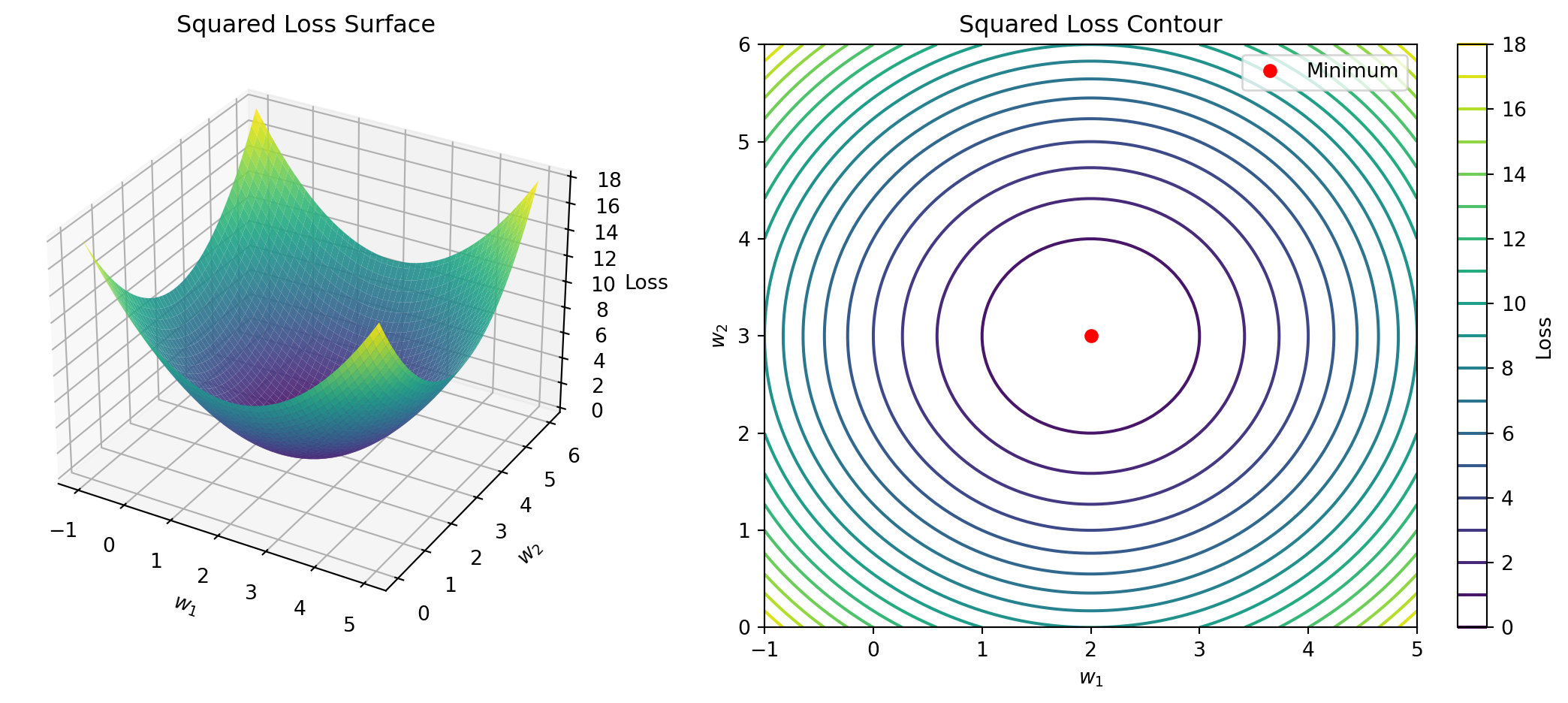
Illustration of Regularization
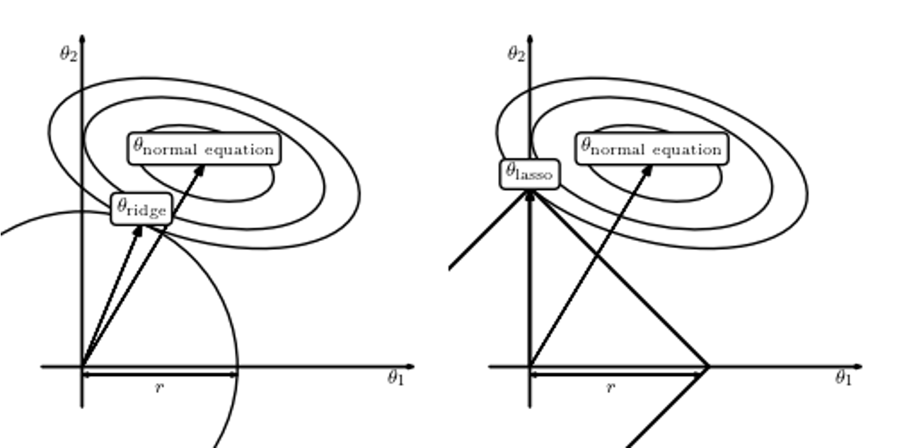
Image source: “Statistics, Data Mining, and Machine Learning in Astronomy” (2013)
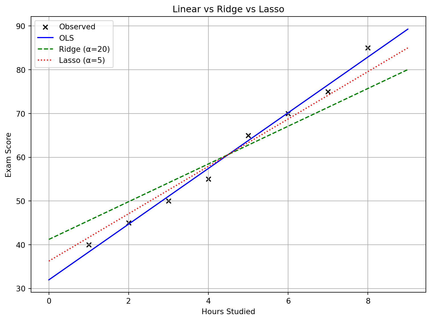
Regularization in Action
We’ll compare three fits on the Hours Studied → Exam Score data:
- Ordinary Least Squares (OLS)
- Ridge Regression (L2, α = 20)
- Lasso Regression (L1, α = 5)
Notice how Ridge smooths (shrinks weights) and Lasso can push weights toward zero.
Comparison