ML Foundations

CISC 484/684 – Introduction to Machine Learning

Author

Affiliation

Sihan Wei

University of Delaware

Published

June 12, 2025

Quick Updates

Final exam:
- Time: 08/15/2025, 4:30PM - 6:30PM
- Location: SHL 105
- The last day of class will be a final review
Canvas course page published (questions?)
HW 1 will be out tonight

Recall

What is Machine Learning?

A set of methods that can automatically detect patterns in data.
Use uncovered patterns to predict future data.
Core components:
- Data
- Model / Hypothesis
- Algorithm to fit the model to data

When Should We Use ML?

Problem is well defined.
No deterministic/rule-based solution.
Have large amounts of high-quality data.
Evaluation is clear and meaningful.

Genres of Machine Learning

Supervised Learning (with labels)
- Regression: continuous labels
- Classification: discrete labels
Unsupervised Learning (without labels)
Semi-supervised Learning (partially labeled data — not covered in this course)
Reinforcement Learning (learning from interaction — not covered in this course)

Setup

Fundamental Assumption in Machine Learning

i.i.d. assumption: data are independent and identically distributed
- Independence: each data point is assumed to be unrelated to others
- Identical distribution: all data points are drawn from the same underlying probability distribution

Formal Setup

Input space: \(\mathcal{X}\) (features)
Output space: \(\mathcal{Y}\) (labels or targets)
Unknown joint distribution: \(p(\mathbf{x}, y)\) over \(\mathcal{X} \times \mathcal{Y}\)
We are given a training set of \(N\) labeled examples:
\[ (\mathbf{x}_i, y_i), \quad i = 1, \ldots, N \] where each pair is drawn i.i.d. from \(p\);
\(\mathbf{x}_i \in \mathcal{X}\), \(y_i \in \mathcal{Y}\)
Goal: Learn a function \(f: \mathcal{X} \rightarrow \mathcal{Y}\) that accurately predicts \(y\) for unseen \(\mathbf{x} \sim p\)

A Familiar Example

Suppose you’re building a system to predict student exam scores based on how many hours they studied. This is a classic example of a supervised learning problem.

Input: hours studied → \(x\)
Output: exam score → \(y\)

We collect training data in the form of:

\[ \{(x^{(1)}, y^{(1)}),\ (x^{(2)}, y^{(2)}),\ \dots,\ (x^{(n)}, y^{(n)})\} \]

Our goal is to learn a function that maps new values of \(x\) (study time) to predicted scores \(y\).

The Learning Problem

Given data:

\[ \{(x^{(i)}, y^{(i)})\}_{i=1}^n \]

we want to learn a function \(h(x)\) such that:

\[ h(x) \approx y \]

\(h(x)\): prediction made by the model
\(y\): the true label (possibly noisy)

The Role of the Hypothesis

We call the function we learn the hypothesis, \(h\):

It’s our best guess of the true function
It’s trained by minimizing a loss on data

The ultimate goal is not to memorize \(y\), but to generalize well to new (unseen) \(\mathbf{x}\).

Modeling Assumption

In supervised learning, we often assume:

\[ y = f(x) + \epsilon \]

Where:

\(f(x)\): the true underlying relationship between input \(x\) and output \(y\) (unknown and possibly unknowable)
\(y\): the observed label (often noisy)
\(\epsilon\): random noise (e.g., measurement error, unobserved variables)
\(h(x)\): our learned model — an approximation of \(f(x)\)

Common Sources of Noise

The noise term \(\epsilon\) captures uncertainty and unmodeled influences, such as:
- Measurement or sensor errors
- Missing or unobserved variables
- Inherent randomness in the environment or process

More About the Noise Term

We typically assume the noise \(\epsilon\) satisfies:
- Zero mean (white noise): \(\mathbb{E}[\epsilon \mid x] = 0\)
- Why?
Sometimes, we also assume: \[ \epsilon \sim \mathcal{N}(0, \sigma^2) \]
- Not necessary, helpful for analysis.
Without the zero-mean assumption, the model would be learning a systematically biased target.

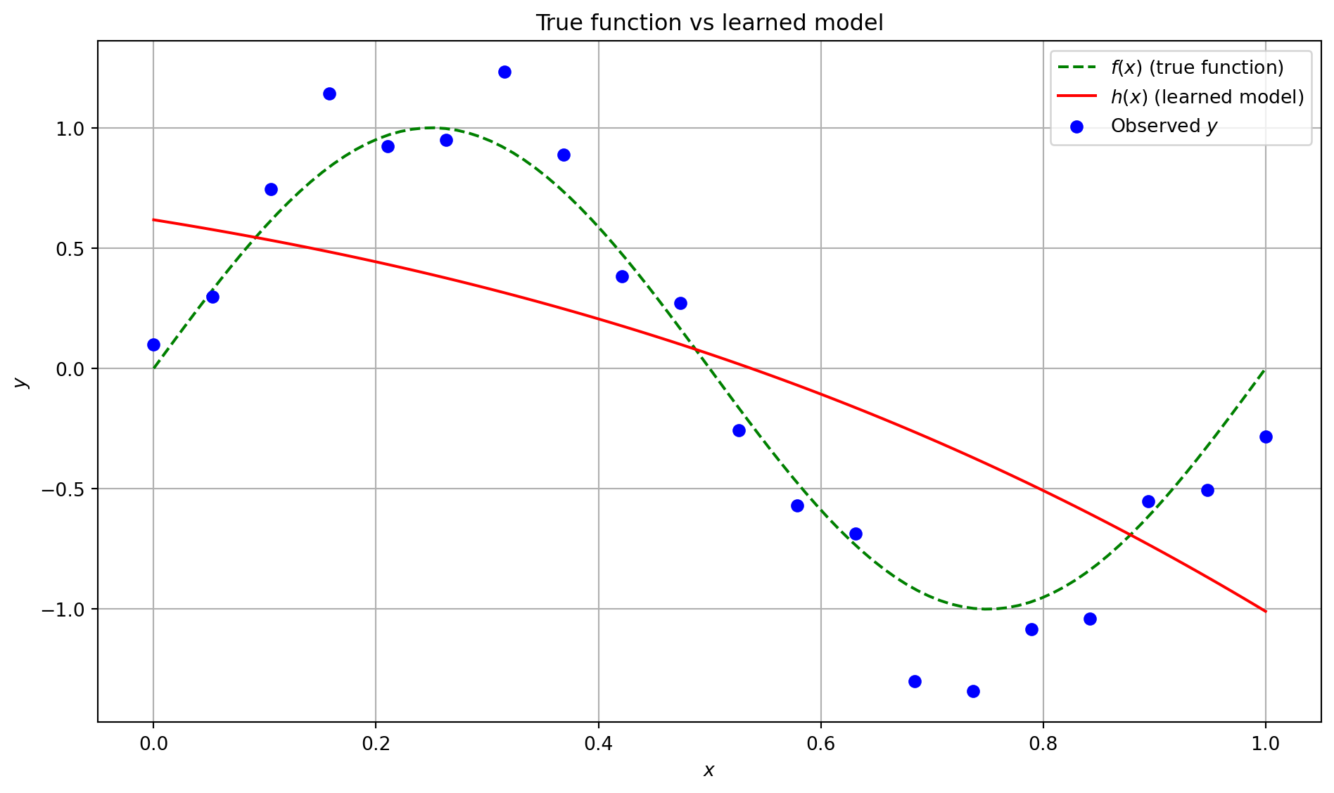
Our Hypothesis \(h(x)\)

We don’t know \(f(x)\), but we learn a model \(h(x)\)
We assume:

\[ y = f(x) + \epsilon \quad \Rightarrow \quad \mathbb{E}[y \mid x] = f(x) \]

So we train \(h(x)\) to minimize the difference from \(y\), hoping:

\[ h(x) \approx f(x) \]

Visualization

Hypothesis Class

Motivation: Why Do We Need Hypothesis Classes?

Before we can learn a function \(h\), we must define what kind of functions we are willing to consider.
- Linear functions? Neural networks? Decision trees? Polynomials?

Motivation Cont’d

Specifying a hypothesis class means choosing a set of allowable functions.
- This encodes our assumptions about the structure of the problem.
- It also determines what the learning algorithm can possibly discover.

Definition: Hypothesis Class

A hypothesis class is the set of functions that a learning algorithm can search over.
It defines the space of possible models we allow during training.
Example (linear regression):
The hypothesis class is all linear functions of the form:
\[ f(x) = w^T x \]

Choosing a Hypothesis Class

A rich hypothesis class is highly expressive, but may overfit the training data.
A simple hypothesis class is easier to learn and generalize from, but may underfit the true pattern.
The goal is to choose a class that:
- Is expressive enough to contain a good (or optimal) solution
- Is simple enough to avoid overfitting and enable efficient learning

Hypothesis Class Tradeoff

Loss Functions

What Is a Loss Function?

A loss function quantifies how “bad” a prediction is — it measures the discrepancy between the predicted output \(h(x)\) and the true label \(y\).
Formally, it’s a function: \[ \ell(h(x), y) \in \mathbb{R}_{\geq 0} \] where smaller values indicate better predictions.

Why Do We Need It?

It gives the learning algorithm a goal: minimize the total (or average) loss over the training data.
Without a loss function, we wouldn’t have a way to compare different hypotheses \(h\).
Different tasks (regression, classification) use different loss functions tailored to the nature of the output and the goal.

0-1 Loss

The 0-1 loss measures whether a prediction is correct or not:

\[ \ell_{0-1}(h(x), y) \stackrel{\text{def}}{=} \begin{cases} 0 & \text{if } h(x) = y \\ 1 & \text{if } h(x) \neq y \end{cases} \]

Common in classification tasks
Easy to interpret, but hard to optimize directly (non-convex, non-differentiable)

Squared Loss

The squared loss measures the squared difference between the prediction and the true label:

\[ \ell_{\text{sq}}(h, (x, y)) = (h(x) - y)^2 \]

Commonly used in regression tasks
Penalizes larger errors more heavily than smaller ones
Differentiable and convex — easy to optimize with gradient-based methods

Why Use Squared Loss?

Assumes that errors (noise) are zero-mean and symmetric — often modeled as Gaussian
Leads to the mean squared error (MSE) objective: \[ \frac{1}{n} \sum_{i=1}^n (h(x^{(i)}) - y^{(i)})^2 \]
The optimal predictor under squared loss is the conditional mean: \[ h^*(x) = \mathbb{E}[y \mid x] \]

Risk

Risk: What Are We Minimizing?

Once we define a loss function \(\ell(h(x), y)\), we can define the total “badness” of a predictor \(h\).
The expected (generalization) risk is the average loss over the true data distribution \(p(x, y)\):

\[ R(h) = \mathbb{E}_{(x, y) \sim p}[\ell(h(x), y)] \]

This is what we really care about: how well does \(h\) perform on future, unseen data?

Empirical Risk

But we don’t know the true distribution \(p(x, y)\)!
Instead, we minimize the empirical risk — the average loss over the training data:

\[ \hat{R}(h) = \frac{1}{n} \sum_{i=1}^{n} \ell(h(x^{(i)}), y^{(i)}) \]

This is computable — and what training algorithms actually minimize.
Empirical Risk Minimization (ERM): \[ h^* = \arg\min_h \hat{R}(h) \]

Why This Matters

Good performance on training data (\(\hat{R}(h)\)) does not guarantee good performance on test data (\(R(h)\)).
The gap between \(R(h)\) and \(\hat{R}(h)\) is called the generalization gap.
Goal: design learning algorithms and hypothesis classes so that this gap is small.

Generalization: The Ultimate Goal

A good model should not just perform well on training data, but also on unseen data.
Generalization = small gap between:
- Empirical risk \(\hat{R}(h)\) (on training set)
- True risk \(R(h)\) (on the data distribution)
Generalization is what separates learning from memorization.

Hoeffding’s Inequality

Let \(h\) be a fixed hypothesis and assume: - Loss \(\ell(h(x), y) \in [0, 1]\) - \((x^{(i)}, y^{(i)})\) are drawn i.i.d. from distribution \(p(x, y)\)

Then, Hoeffding’s inequality says:

\[ \Pr\left( \left| R(h) - \hat{R}(h) \right| \geq \gamma \right) \leq 2 \exp(-2n\gamma^2) \]

\(R(h)\) = true risk
\(\hat{R}(h)\) = empirical risk
\(n\) = number of training examples
\(\gamma\) = generalization gap

Interpretation

With high probability, the empirical risk is close to the true risk.
As \(n\) increases, the probability of a large generalization gap shrinks exponentially.
This holds for a fixed hypothesis \(h\).

But what if we choose \(h\) after seeing the data? → Let’s talk about uniform convergence next.

Uniform Convergence

To guarantee generalization for all hypotheses in a finite class \(\mathcal{H}\), we use the union bound:

\[ \Pr\left( \exists h \in \mathcal{H}: |R(h) - \hat{R}(h)| \geq \gamma \right) \leq 2 |\mathcal{H}| \cdot \exp(-2n\gamma^2) \]

The probability that any hypothesis in \(\mathcal{H}\) has large error is bounded.
As \(|\mathcal{H}|\) increases, the bound gets looser.

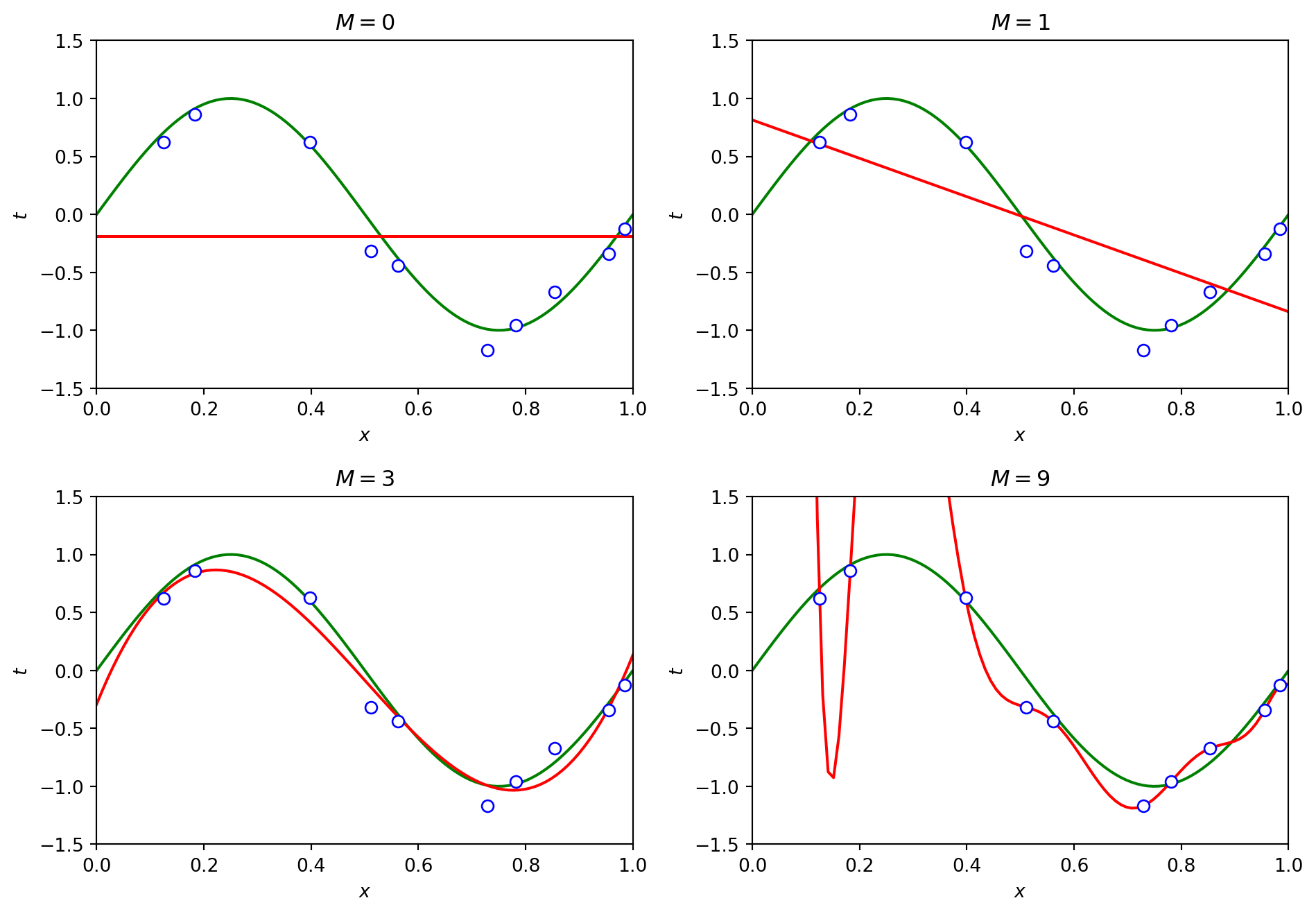
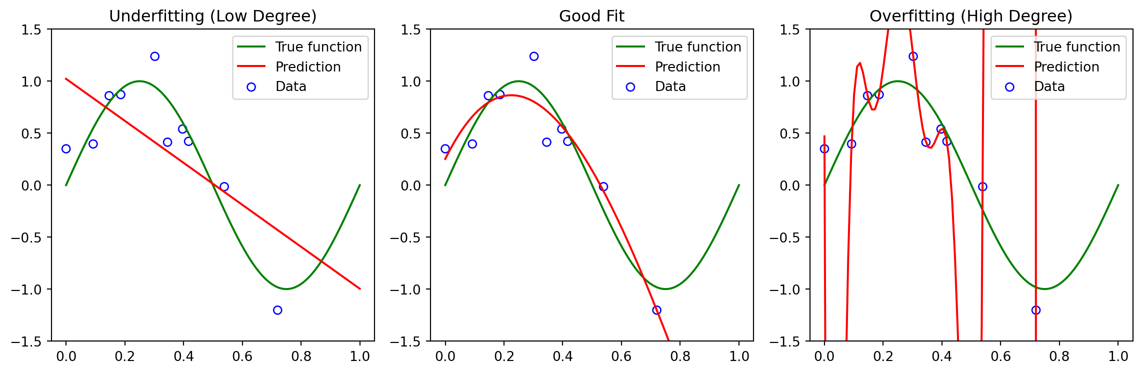
Underfitting vs Overfitting

Underfitting:
- Model is too simple to capture patterns in the data
- High training error and high test error
Overfitting:
- Model is too complex, learns noise in the training data
- Low training error, but high test error
Goal: Find a model that generalizes well

Bad Example: The “Memorizer”

Consider a function \(h(\cdot)\) that simply memorizes the training data \(D\):

\[ h(x) = \begin{cases} y_i, & \text{if } \exists (x_i, y_i) \in D \text{ such that } x = x_i \\ 0, & \text{otherwise} \end{cases} \]

This \(h(\cdot)\) achieves 0% training error
But it performs poorly on unseen data
It doesn’t generalize — it overfits by memorizing specific examples

Visualizing the Tradeoff

Bias vs Variance

Where Does Error Come From?

We can break the expected squared error at a point \(x\) into three components:

\[ \begin{split} \mathbb{E}_{\mathcal{D}}[(h_{\mathcal{D}}(x) - y)^2] &= \underbrace{(\mathbb{E}_{\mathcal{D}}[h_{\mathcal{D}}(x)] - f(x))^2}_{\text{Bias}^2} \\ &+ \underbrace{\mathbb{E}_{\mathcal{D}}\left[(h_{\mathcal{D}}(x) - \mathbb{E}_{\mathcal{D}}[h_{\mathcal{D}}(x)])^2\right]}_{\text{Variance}} \\ &+ \underbrace{\mathbb{E}[(y - f(x))^2]}_{\text{Noise}} \end{split} \]

\(h_{\mathcal{D}}(x)\) is the model trained on dataset \(\mathcal{D}\)
\(f(x)\) is the true function
\(y = f(x) + \epsilon\), and \(\epsilon\) is zero-mean noise

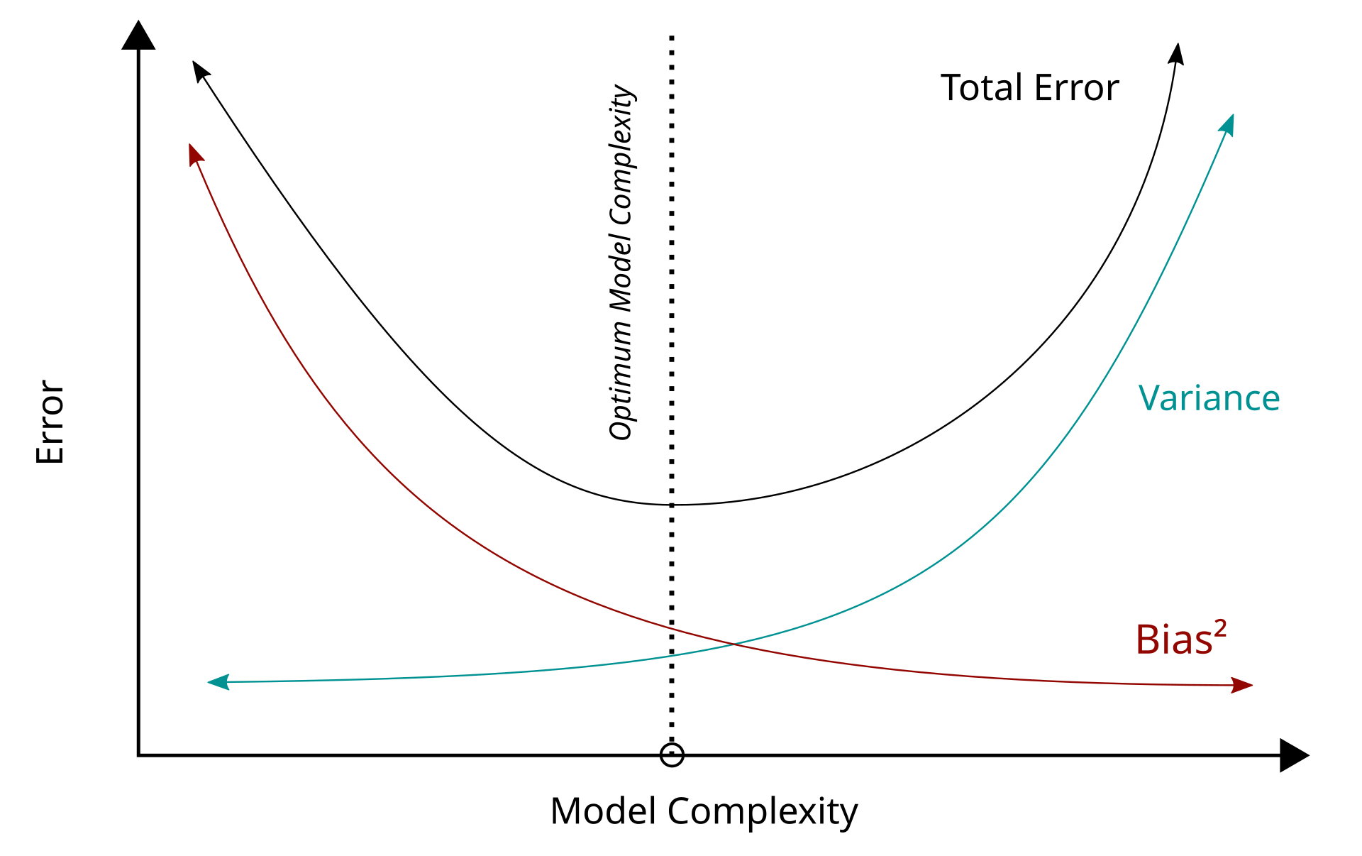
Bias–Variance Tradeoff

Bias: Error from wrong assumptions (e.g., model too simple)
- High bias ⇒ underfitting
Variance: Error from sensitivity to training data
- High variance ⇒ overfitting
Noise: Irreducible randomness in the data-generating process
We want to find the sweet spot between bias and variance.

Model Complexity and Error

As model complexity increases:
- Bias decreases: the model can fit the true function better
- Variance increases: the model reacts more to noise in the training data
The goal is to minimize the total expected error: \[ \text{Total Error} = \text{Bias}^2 + \text{Variance} + \text{Noise} \]

This is why regularization, cross-validation, and careful model selection matter!

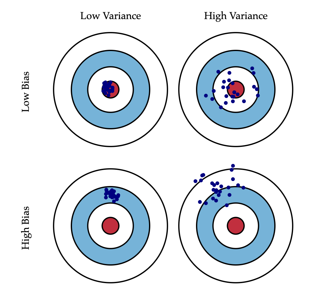
Bias-variance tradeoff

Regularization

What Is Regularization?

Instead of minimizing empirical risk alone: \[ \hat{R}(h) = \frac{1}{n} \sum_{i=1}^n \ell(h(x^{(i)}), y^{(i)}) \]
We minimize the regularized objective: \[ \hat{R}_{\text{reg}}(h) = \hat{R}(h) + \lambda \cdot \Omega(h) \]
- \(\Omega(h)\): complexity penalty
- \(\lambda\): regularization strength (hyperparameter)

Why Regularization Helps

Controls model complexity without needing to change the hypothesis class
Helps prevent overfitting (high variance)
May introduce bias, but reduces variance — often leads to better generalization
Think of it as “tugging the model toward simplicity”

Common Regularization Techniques

L2 regularization (Ridge): \[ \Omega(h) = \|w\|_2^2 \quad \text{→ encourages small weights} \]
L1 regularization (Lasso): \[ \Omega(h) = \|w\|_1 \quad \text{→ encourages sparsity (some weights = 0)} \]
Can apply to:
- Linear regression and logistic regression
- Neural networks
- Other parameterized models

Regularization Tradeoff

Small \(\lambda\):
- Weak regularization → model may overfit
Large \(\lambda\):
- Strong regularization → model may underfit
Choose \(\lambda\) using validation data or cross-validation

Visualization

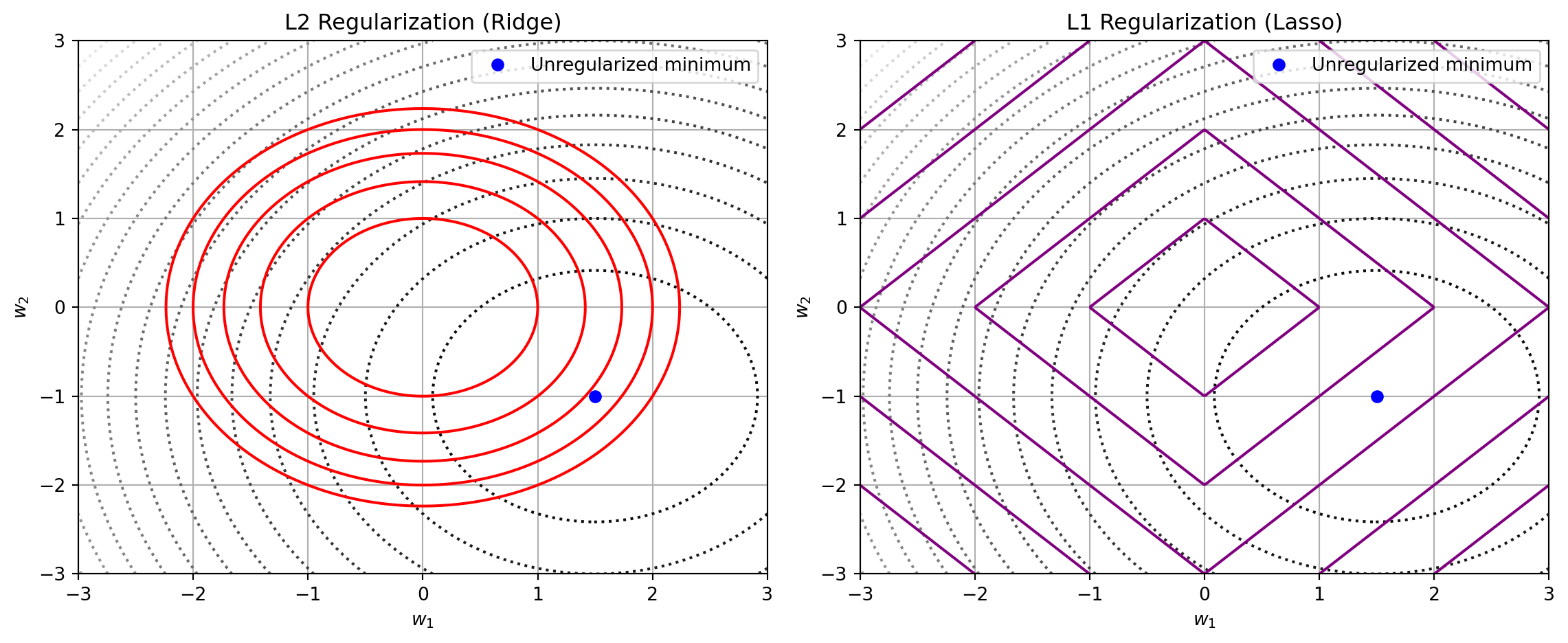
L1 vs L2 Regularization: Comparison

Feature	L1 (Lasso)	L2 (Ridge)
Penalty term	\(\lambda \\|w\\|_1 = \lambda \sum \|w_i\|\)	\(\lambda \\|w\\|_2^2 = \lambda \sum w_i^2\)
Geometry	Diamond-shaped contours	Circular contours
Solution behavior	Sparse: some \(w_i = 0\)	Shrinks all weights smoothly
Feature selection	Yes — performs automatic selection	No — retains all features
Optimization	Non-differentiable at 0 (but convex)	Differentiable and convex

L1 vs L2 Cont’d

L1: encourages sparsity → good for interpretability and feature selection
L2: discourages large weights → good for generalization and numerical stability